11 Tree-based Models
\[\def\1{\unicode{x1D7D9}}\]
In the previous chapter, we used the tidymodels package to build a classification model for the titanic data set from the infamous kaggle competition of the same name. More precisely, we
- split our data for training and testing purposes,
- handled all pre-processing steps by using a recipe,
- used logistic regression to implement our model specification and
- used a workflow to coordinate all of these parts.
Due to this compartmentalization of tasks you may suspect that the previous steps can be easily adapted to accommodate different model specification, e.g. if we want to move away from using a logistic regression.
Luckily, this is exactly the case.
To change our model, we have to only tweak the model specification and possibly add or remove a few preprocessing steps, e.g. those that were added only for technical reasons like step_zv().
In this chapter, we want to introduce a new model specification. Specifically, we want to use a tree-based model called random forest. Even without knowing how this model works, we can state that what we need to change compared to our calculations from the last chapter requires us to
- change the ‘standard technical steps’ for logistic regression to those of random forests and
- change the model specification.
This is done as follows. Notice that most of the code is simply copied from the previous chapter.
library(tidyverse)
library(tidymodels)
############# Read data and label outcome
titanic <- read_csv("data/titanic.csv")
titanic <- titanic %>%
  mutate(
    Survived = factor(
      Survived,
      levels = c(0,1),
      labels = c("Deceased", "Survived")
    )
  )

############# Data Splitting stays the same
set.seed(123)
titanic_split <- initial_split(titanic, strata = Survived)
titanic_train <- training(titanic_split)
titanic_test <- testing(titanic_split)
set.seed(456)
titanic_folds <- vfold_cv(titanic_train, strata = Survived)


############# Change only technical recipe steps
titanic_rec <- recipe(formula = Survived ~ ., data = titanic_train) %>%
  ### Our pre-processing from the previous analysis
  update_role(PassengerId, new_role = "Id") %>%
  step_mutate(Cabin = if_else(is.na(Cabin), "Missing", "Available")) %>%
  step_impute_median(Age) %>%
  step_mutate(
    title = str_match(Name, ", ([:alpha:]+)\\."),
    title = if_else(is.na(title[, 2]), "NA", title[, 2])
  ) %>%
  step_other(title, threshold = 0.02, other = "Other") %>%
  step_rm(Ticket, Embarked) %>%
  update_role(Name, new_role = "Id") %>%
  ### Leave only one "technical step"
  step_string2factor(all_nominal_predictors())

############# New model specification
############# tune() explained in a sec
titanic_spec <-
  rand_forest(mtry = tune(), min_n = tune(), trees = 1000) %>%
  set_mode("classification") %>%
  set_engine("ranger")

############# Workflow stays the same
titanic_wf <- workflow() %>%
  add_recipe(titanic_rec) %>%
  add_model(titanic_spec)
As you can see from this, random forest can be considered as “low maintenance models” as they require only very little technical preprocessing steps.
Further, you may have noticed that the new model specification uses (cryptic) arguments mtry, min_n and trees in conjunction with a function tune().
This function is used to let the recipe know which of those so-called hyperparameters mtry, min_n and trees of the random forest model will be tuned with help from the data, i.e. not set manually.
However, before we do that, it is probably a good idea to learn more about random forests in order to understand what those hyperparameters even mean.
11.1 Random Forests
Like any forest, random forests consist of a lot of different trees. In our case, these trees will be so-called (random) decision trees. Fundamentally, you can imagine a decision tree as a construct that uses simple decision rules repeatedly until one arrives at a conclusion.
For instance, take a look at the following fictitious decision tree. Using this tree it is possible to classify a person as either not a Taylor Swift fan, a regular Taylor Swift fan or a true Swiftie based on the numbers of Taylor Swift songs one listened too recently and the number of Taylor Swift concerts one attended.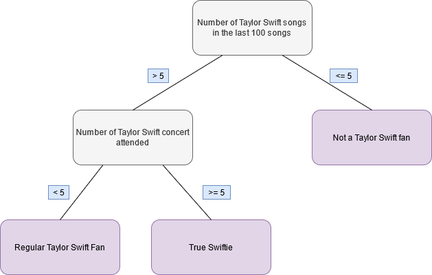
Figure 11.1: Fictitious decision tree to classify Taylor Swift fans
So if we wanted to classify a person using this tree, then all we have to do80 is follow along the lines from the tree root (here the number of songs) to one of the tree’s terminal nodes (in red-ish).
Thus, using a data set to fit a decision tree for classification, aka a classification tree, is a matter of finding variables within this data set that serve well as internal nodes in a tree in conjunction with appropriate splitting points of that variable. In order to understand what kind of procedure can find these things for us, let us look at regression trees first.
This is possible because the terminal nodes of a tree do not have to be categorical variables but can be numerical constants too.
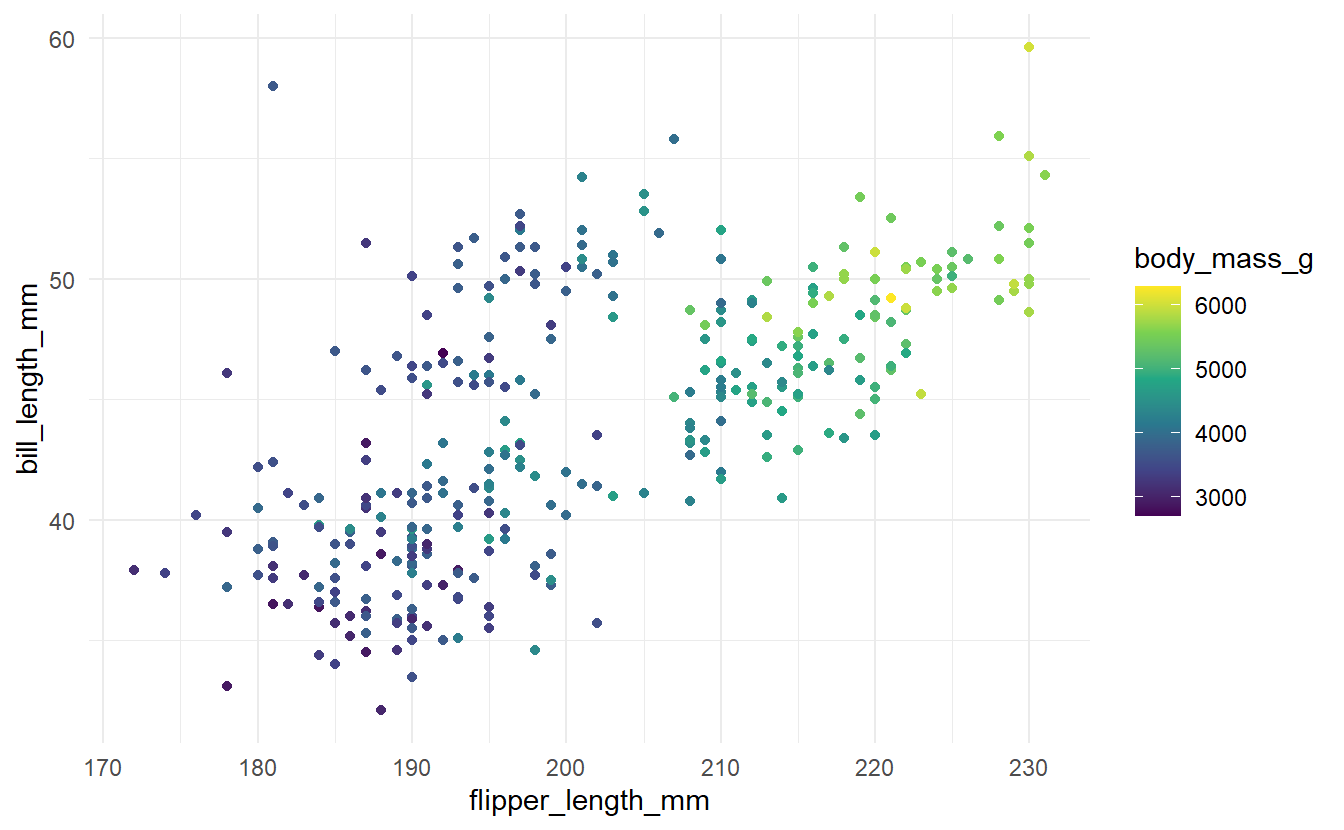
For instance, take a look at the palmerpenguins package that contains different measurements of penguins from Palmer Archipelago.
library(palmerpenguins)
penguins <- penguins %>% na.omit()
Here, we could fit a decision tree that tries to explain body_mass_g (a numerical variable) via flipper_length_mm and bill_length_mm.
So, we will try to fit a model to the following data.
penguins %>%
  ggplot(aes(x = flipper_length_mm, y = bill_length_mm)) +
  geom_point(aes(col = body_mass_g)) +
  theme_minimal() +
  scale_colour_viridis_c(
    limits = range(penguins$body_mass_g, na.rm = TRUE),
    aesthetics = c('colour', 'fill')
  )
Now, what a decision tree fundamentally tries to do is to split the space spanned by the predictors into regions \(R_1, \ldots, R_n\) and assign constant values \(c_1, \ldots, c_n\) to each region in the hope that all observed response values in a given region \(R_i\) are actually close to the corresponding constant \(c_i\).
Finally, before we move on to find out how these regions and constants are determined let us see the result in action first.
In R, a decision tree can be easily fit using rpart() from the package of the same name.
Also, the result can be neatly visualized using geom_parttree() from the parttree package.
library(rpart)
library(parttree)
tree <- rpart(data = penguins, body_mass_g ~ flipper_length_mm + bill_length_mm)

ggplot(data = penguins, aes(x = flipper_length_mm, y = bill_length_mm)) +
  geom_parttree(data = tree, aes(fill=body_mass_g), alpha = 0.3) +
  geom_point(aes(col = body_mass_g)) +
  theme_minimal() +
  scale_colour_viridis_c(
    limits = range(penguins$body_mass_g, na.rm = TRUE),
    aesthetics = c('colour', 'fill')
  )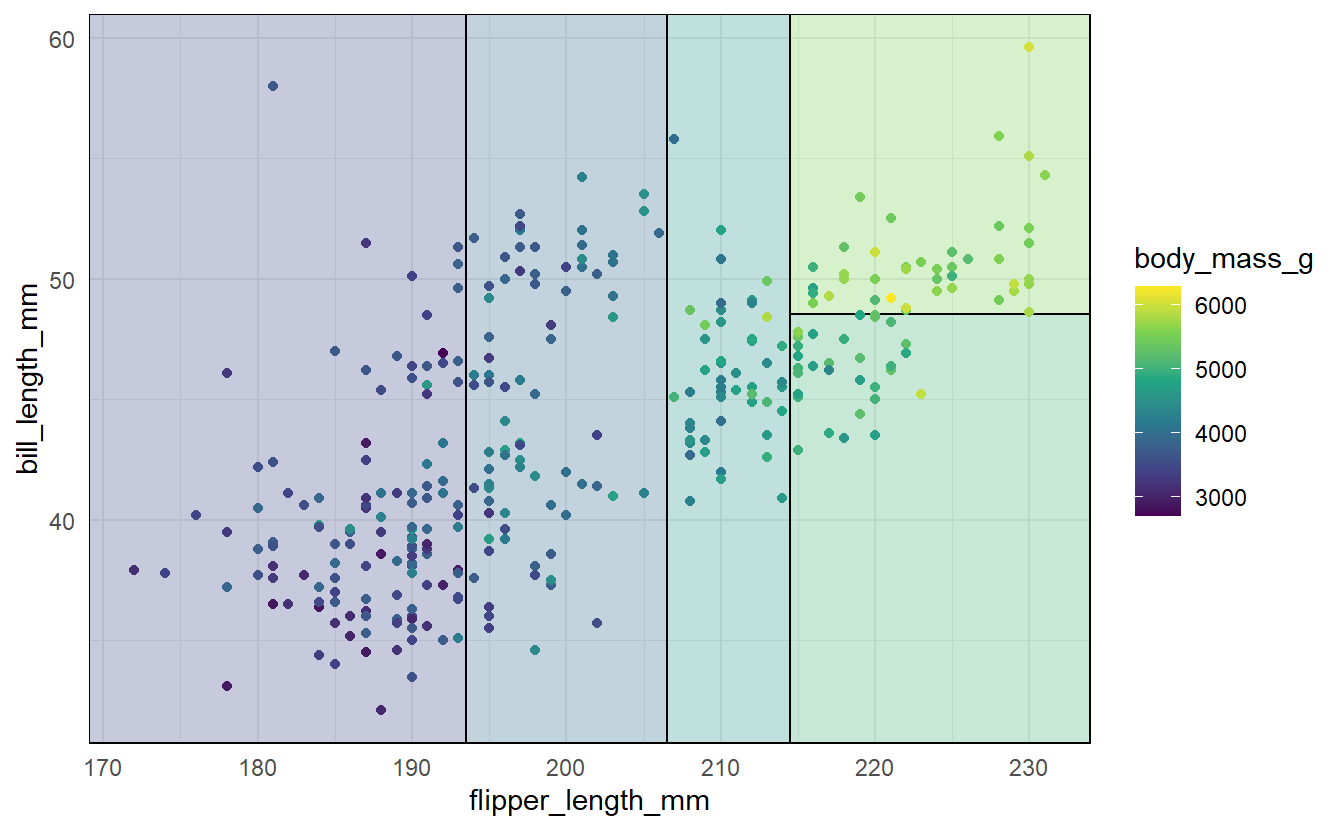
As you can see here, the plane that was spanned by flipper_length_mm and bill_length_mm was split into 5 regions which were each assigned a constant (as indicated by each region’s shading).
11.1.1 How to Build a Tree
As we have seen in the penguins example, a regression tree predicts a response \(Y\) based on \(n\) predictors by finding a number of regions \(R_i \subset \mathbb{R}^n\) with constants \(c_i\), \(i = 1, \ldots, M\), such that the predicted response \(\hat{Y}\) is given by \[\begin{align*} \hat{Y} = f(X_1, \ldots, X_n) = \sum_{i = 1}^{M}c_i \1\{ (X_1, \ldots, X_n) \in R_i \}, \end{align*}\] where \(M\) describes the number of regions that were found by a tree-building algorithm.
In order to build a tree the first step is to split the data that is being fitted into two. This way we go from a tree that only contains a single node, namely its root, to a tree that has one split, i.e. the tree has a one root and two terminal nodes. Once we are able to do that we can iteratively split the terminal nodes further.
If you have trouble imagining this, you may also think of the spanned space of all predictors instead. Actually, this first splitting step is akin to splitting the space that is spanned by all predictors, say \(\tilde{R}_0\), into two regions \(\tilde{R}_1\) and \(\tilde{R}_2\). Then, one may take one of those two new regions, say \(\tilde{R}_1\) and split that into two again, say \(\tilde{R}_3\) and \(\tilde{R}_4\) and so on. This whole procedure can then be done until a region contains only a minimal amount of observations, say 5, which is when the splitting stops. The final regions \(R_1, \ldots, R_M\) are then given by the partition of the \(\tilde{R}_0\) that is present once the splitting procedure stops.
Of course, this begs the question of how an algorithm determines how to split the regions. As we have seen in the previous examples, for a decision tree the splitting rule is somewhat simple: A region \(R\) is split into two parts \(R_1\) and \(R_2\) based on a single predictor denoted by, say, \(X_j\) and a splitting point \(s\) via \[\begin{align*} R_1(j, s) = \{ X \vert X_j \leq s \} \quad \text{ and } \quad R_2(j, s) = \{ X \vert X_j > s \}. \end{align*}\] Here, we have assumed that \(X_j\) is a numerical predictor. For categorical predictors the splitting rule is done similarly though requires some additional considerations beforehand81.
Now, to determine what splitting variable \(X_j\) and splitting point \(s\) to use, we need to consider that each new region \(R_1(j, s)\) and \(R_2(j, s)\) is also assigned a constant \(c_1\) and \(c_2\) that is later used for prediction if a region is not split further. Thus, an algorithm may be implemented that chooses \(j, s, c_1\) and \(c_2\) in such a way that the regression error will be minimal if the tree is not split any further.
In order to implement this we need to determine some measure \(Q_R(R, c)\), which is sometimes referred to as node impurity measure, that gives us feedback on the regression error given a region \(R\) and associated constant \(c\). An obvious choice would be to use the sum of squared residuals (SSR), i.e. \[\begin{align*} Q_R(R, c) = \sum_{x_i \in R} (y_i - c)^2. \end{align*}\] Obviously, given a region \(R\) the SSR is minimal if \(c\) is the average of response variables \(y_i\) in \(R\). Therefore, we can consider one less variable to optimize by simply considering only \[\begin{align*} Q_R(R) = \sum_{x_i \in R} (y_i - \hat{c}(R))^2 \end{align*}\] as measure of our regression error where \(\hat{c}(R)\) denotes the average of the response variable in the region \(R\).
Consequently, using this measure \(Q\), we can determine the splitting variable \(X_j\) and splitting point \(s\) by simply scanning through all possibilities in order to solve the minimization problem \[\begin{align*} \min_{j, s} \Big( Q_R\big(R_1(j, s)\big) + Q_R\big(R_2(j, s)\big) \Big). \end{align*}\]
Again, this splitting and optimization procedure is repeated until another splitting becomes unfeasible because the new regions would contain less observations than some minimal amount we need specify.
In essence, this is what the min_n argument in rand_forest() is controlling and because different values for min_n may yield different trees, we may try to optimize this argument via tuning.
Further, let us talk about how to adjust this tree building procedure for classification purposes. Notice that the only instance where our procedure relied on the fact that our response observations \(y_i\) were numerical is when evaluating the regression error via the node impurity measure.
Previously, the numerical nature of \(y_i\) allowed us to use the sum of squared residuals node impurity measure \(Q_R\). However, this is clearly not an appropriate choice when the responses \(y_i\) are categorical. Therefore, we will need to use a more appropriate measure for categorical responses.
One such measure is given by the Gini impurity measure \[\begin{align*} Q_R(R) = \sum_{k=1}^{K} \hat{p}(R, k)(1 - \hat{p}(R, k)), \end{align*}\] where \(K\) is the number of levels of the response variable \(Y\) and \(\hat{p}(R, k)\) describes the proportion of class \(k\) observations in region \(R\). Here, it might be confusing to not see a sort of comparison between predicted and observed class similar to our previous impurity measure.
This is why it helps to consider the following scenario. Imagine that given a region \(R\) we would classify any observation in \(R\) randomly according to the distribution of classes in \(R\), i.e. any observation in R is classified as being of class \(k\) with probability \(\hat{p}(R, k)\). Then, via a simple argument using the law of total probability we can compute the probability of \(A\) which describes the event that “a randomly chosen observation from \(R\) is classified incorrectly”. Letting \(B\) denote the class of the randomly chosen observation, \(\mathbb{P}(A)\) is given by \[\begin{align*} \mathbb{P}(A) = \sum_{k = 1}^{K} \mathbb{P}(A \vert B = k) \mathbb{P}(B = k) = \sum_{k=1}^{K} \hat{p}(R, k)(1 - \hat{p}(R, k)), \end{align*}\] which is exactly the Gini impurity measure.
Thus, this measure quantifies in a specific region \(R\) how often a randomly chosen element would be labeled incorrectly if it was randomly assigned a class label according to the label distribution within \(R\). Finally, once regions have been determined, all observations in a given region are labeled according to a majority vote, i.e. all observations in \(R\) are labeled as being of class \(k\) that maximizes \(\hat{p}(R, k)\).
11.1.2 How to Choose a Tree
The previous description allowed us to understand how we can sequentially split our space spanned by the predictors into ever smaller regions until the regions would become too small to split further. This gives us a sequence of sets of regions from a space that is not split at all (one region) to a space that is split a lot (many regions). Similarly, this gives us a sequence of corresponding trees.
Once a full-sized tree has been determined from the data set, it becomes time to consider whether we actually want our decision tree to be full-sized. Fundamentally, this comes down to trying to prevent overfitting because a full-sized tree might split the data into way too many regions such that the tree loses its predictive power for unseen data. Therefore, we might want to use one of our intermediate trees in our sequence of trees that we obtained as part of our splitting procedure.
But in order to decide which of those trees we should use we again need some measure that evaluates a tree. Now, this measure should take into account not only our previous impurity measure \(Q_R\) but also the size of the tree / the number of regions. This defines the cost complexity criterion of a tree \(T\) \[\begin{align*} C_{\alpha}(T) = \sum_{i = 1}^{\vert T \vert} Q_R(R_i) + \alpha\vert T\vert, \end{align*}\] where \(R_i\) correspond to the \(i\)-th region of a tree \(T\) with \(\vert T \vert\) terminal nodes and \(\alpha \geq 0\) is a tuning parameter governing the trade-off between size and impurity.
Moreover, depending on \(\alpha\) each tree along our sequence of trees may have a different cost complexity value. Clearly, for \(\alpha = 0\), the tree with the lowest cost complexity value will be the full-sized tree because by construction this tree minimizes the total impurity \(\sum_{i = 1}^{\vert T \vert} Q_R(R_i)\). This is due to the fact that the the splitting procedure minimizes the total impurity, i.e. as the tree becomes larger the total impurity becomes smaller.
However, when \(\alpha > 0\), then large trees are penalized for their size and the cost complexity value of large trees may exceed that of smaller trees even though the total impurity of the former is smaller than that of the latter trees. Thus, to fit an “optimal” tree we need to find a suitable value for \(\alpha\) and then take the tree that minimizes the cost complexity value given that \(\alpha\). To keep things short here, let me simply mention that this optimal value of \(\alpha\) can be found using some form of v-fold cross validation82.
11.1.3 How to Build a Random Forest
Once we are able to fit a single tree to one data set, we are also able to fit a lot of trees corresponding to bootstrapped samples of the same underlying data. After that is done and we have fitted, say, 1000 trees we can run a regression/classification based on a set of predictors for each of those 1000 trees. This gives us 1000 estimates that we can combine into a single estimate via averaging (in case of regression) or casting a majority vote (in case of classification).
This kind of ensemble learning, i.e. combining multiple estimates, is known as bagging. Here, bagging refers to specifically the aggregation of bootstrapped estimates but, in general, ensemble learning can use other means of combining multiple estimates. So, in essence, building a random forest is a bagging procedure based on decision trees.
Though, there is one thing that is somewhat special about random forests, namely the tree building procedure is tweaked in order to decorrelate the resulting ensemble of trees. This is motivated by the fact that bagging is mainly a procedure to reduce variance and the fact that the variance of the average of \(N\) identically distributed random variables with pairwise correlation \(\rho \geq 0\) is given by \[\begin{align*} \frac{\sigma^2}{N} + \bigg( 1 - \frac{1}{N} \bigg)\rho \sigma^2. \end{align*}\]
Consequently, only increasing the number of trees \(N\) would mean that the variance reduction is limited by \(\rho\sigma^2\) but if we also manage to decrease the correlation \(\rho\) without compromising the variance \(\sigma^2\) too much, then this will improve our variance reduction even more.
Thus, random forests try to decorrelate the trees.
This is done by considering not all predictors in each tree splitting step but only a random selection of predictors.
Finally, the parameter mtry in rand_forest() determines the number of predictors that are randomly sampled at each splitting step.
11.2 Fitting a Random Forest
Now that we know how to build a random forest, let us finally use our tidymodels workflow to tune the forest’s hyperparameters in order to find an optimal random forest for this data set.
Previously, we set the number of trees in our forest trees to 1000.
Therefore, we only need to tune mtry and min_n.
Here, we simply want to iterate through a set of predetermined possible values of mtry and min_n.
This can be done via tune_grid() but first we need to establish a grid of parameters in order iterate through it83.
titanic_grid <- expand_grid(
  min_n = 5:7,
  mtry = 1:4
)
titanic_grid
#> # A tibble: 12 x 2
#>   min_n  mtry
#>   <int> <int>
#> 1     5     1
#> 2     5     2
#> 3     5     3
#> 4     5     4
#> 5     6     1
#> 6     6     2
#> # ... with 6 more rows
Once a grid is established (here we have simply taken arbitrary values), we can call tune_grid() with our workflow, cross validation folds, grid and a metric set to evaluate the trees.
Additionally, we can control some of tune_grid’s behavior via specifying the control argument by control_grid().
For instance, we could let the tuning process save the predictions of our folds (save_pred = TRUE).
Also, because we will enable parallel processing here to speed up the tuning, we will also need to make sure that any custom pre-processing steps we are using (such as the computation of title) have access to the functions they need.
While this seems obvious, sometimes in preprocessing one has to manually make sure that each “worker” that runs in parallel loads the necessary packages84.
This can be done via pkgs = c(<package names>).
# enable parallel processing on 6 threads to speed up tuning
doParallel::registerDoParallel(cores = 6)
set.seed(14834)
titanic_tune <- tune_grid(
  titanic_wf,
  resamples = titanic_folds,
  grid = titanic_grid,
  metrics = metric_set(sensitivity, specificity, mcc, roc_auc),
  control = control_grid(save_pred = TRUE, pkgs = "tidyverse")
)
Once this computation is complete (which can take a while even with parallel processing enabled via registerDoParallel()), we can look at the best performing hyperparameters w.r.t. a metric we specified earlier.
show_best(titanic_tune, metric = "roc_auc")
#> # A tibble: 5 x 8
#>    mtry min_n .metric .estimator  mean     n std_err .config
#>   <int> <int> <chr>   <chr>      <dbl> <int>   <dbl> <chr>
#> 1     2     6 roc_auc binary     0.879    10  0.0138 Preprocessor1_Model06
#> 2     3     7 roc_auc binary     0.879    10  0.0148 Preprocessor1_Model11
#> 3     3     5 roc_auc binary     0.878    10  0.0148 Preprocessor1_Model03
#> 4     4     5 roc_auc binary     0.878    10  0.0156 Preprocessor1_Model04
#> 5     2     7 roc_auc binary     0.878    10  0.0142 Preprocessor1_Model10
Then, we either manually choose a set of parameters from this list or simply take the parameter that minimizes our metric.
optim_param <- select_best(titanic_tune, metric = "roc_auc")After this is done, we finalize our workflow with these parameters and run our last fit. Last but not least, we can then check the performance of our final model.
titanic_wf <- finalize_workflow(titanic_wf, optim_param)
set.seed(156)
final_rf <- last_fit(titanic_wf, titanic_split)
collect_metrics(final_rf)
#> # A tibble: 2 x 4
#>   .metric  .estimator .estimate .config
#>   <chr>    <chr>          <dbl> <chr>
#> 1 accuracy binary         0.808 Preprocessor1_Model1
#> 2 roc_auc  binary         0.874 Preprocessor1_Model1
11.3 Exercises
11.3.1 Tuning the Amount of Trees
Use mtry = 2 and min_n = 5 to tune the number of trees of our forest, i.e. find the optimal numbers of trees in \(\{1, 2, \ldots, 20, 50, 75, 100, 200, \ldots, 700 \}\) that maximizes the AUC value.
Further, generate a plot that plots the AUC against the number of trees.
Important: Save your variable that is produced bytune_grid() into an RDS-file and push it to your branch so that I do not have to refit your model.
Your final code should include read_RDS(...) and your code that generated the RDS file should be commented out.
11.3.2 Fitting a Decision Tree
Instead of using parsnip::rand_forest() use parsnip::decision_tree() to fit the same model as in the lecture notes only with a different model specification using a single decision tree instead of a random forest.
Tune the parameters tree_depth and min_n and use the default value for cost_complexity.
What is the best AUC value your tuning can produce?85
Important: Save your variable that is produced bytune_grid() into an RDS-file and push it to your branch so that I do not have to refit your model.
Your final code should include read_RDS(...) and your code that generated the RDS file should be commented out.