5 The Monte Carlo Method
\(\def\1{\unicode{x1D7D9}}\) Anyone who has ever taken an elementary problem has probably heard of Buffon’s needle experiment. Basically, this experiment consists of repeatedly throwing a needle on a floor made of parallel strips of wood each of the same width. The aim of the experiment was to measure the probability that the needle will lie across one of the (theoretical) lines of two neighboring strips of wood.
From the strong law of large numbers (SLLN) we know that the sample mean \(\bar{X}_n\) of a sample consisting of independent and identically distributed (iid) random variables \(X_n,\) \(n \in \mathbb{N}\), converges almost surely to \(\mathbb{E}X_1\) iff \(\mathbb{E}\vert X_1 \vert < \infty\). Consequently, the SLLN justifies using the relative frequency of how many times an event \(A\) occurred after \(n\) independent experiments as approximation of the probability of event \(A\). This follows from \(A_k = \text{"A occured in $k$-th trial"}\) and \[\begin{align*} \text{rel. freq.} = \frac{1}{n} \sum_{k = 1}^{n} \1\{A_k\} \rightarrow \mathbb{E}\1\{A_1\} = \mathbb{P}(A) \quad \text{a. s.} \end{align*}\] as \(n \rightarrow \infty\) as per the SLLN.
Therefore, if Buffon counted how many times his thrown needle was lying across a line, then he could compute the relative frequency of this event occurring pretty easily and got an approximation of the probability he was looking for. Of course, this assumes that he has thrown the needle very often. Assuming that no one really wants to throw a needle (or noodle48) thousands of times, this is a good chance for modern computers to step in.
If we can simulate appropriate random numbers that resemble the throwing process, we can let the computer do the “throwing” and counting for us. This, at heart, is what the so-called Monte-Carlo method is all about. To illustrate this, let us look at a maybe even simpler example.
Assume further that we agree to drink said beer in a pub in the city at a not further specified time between 3 and 4 pm and each one of us shows up at that pub independently. Also, each one of us will not show up before 3 pm, is not willing to wait longer than 15 minutes and leaves at 4 pm at the latest. Now, what is the probability that we will actually meet each other under these conditions?
From elementary probability we know that we can compute the exact probability via a geometric approach.
This means that we first think of the vector of possible arrival times \((L, A)\) of Lars \((L)\) and me \((A)\) as points within the square \([0, 60]^2\) (60 as in 60 minutes in an hour).
Then, we will have to compute the area of the square \([0, 60]^2\) which corresponds to the desired event and divide it by the area of the whole square.
In this case, the desired area looks like this
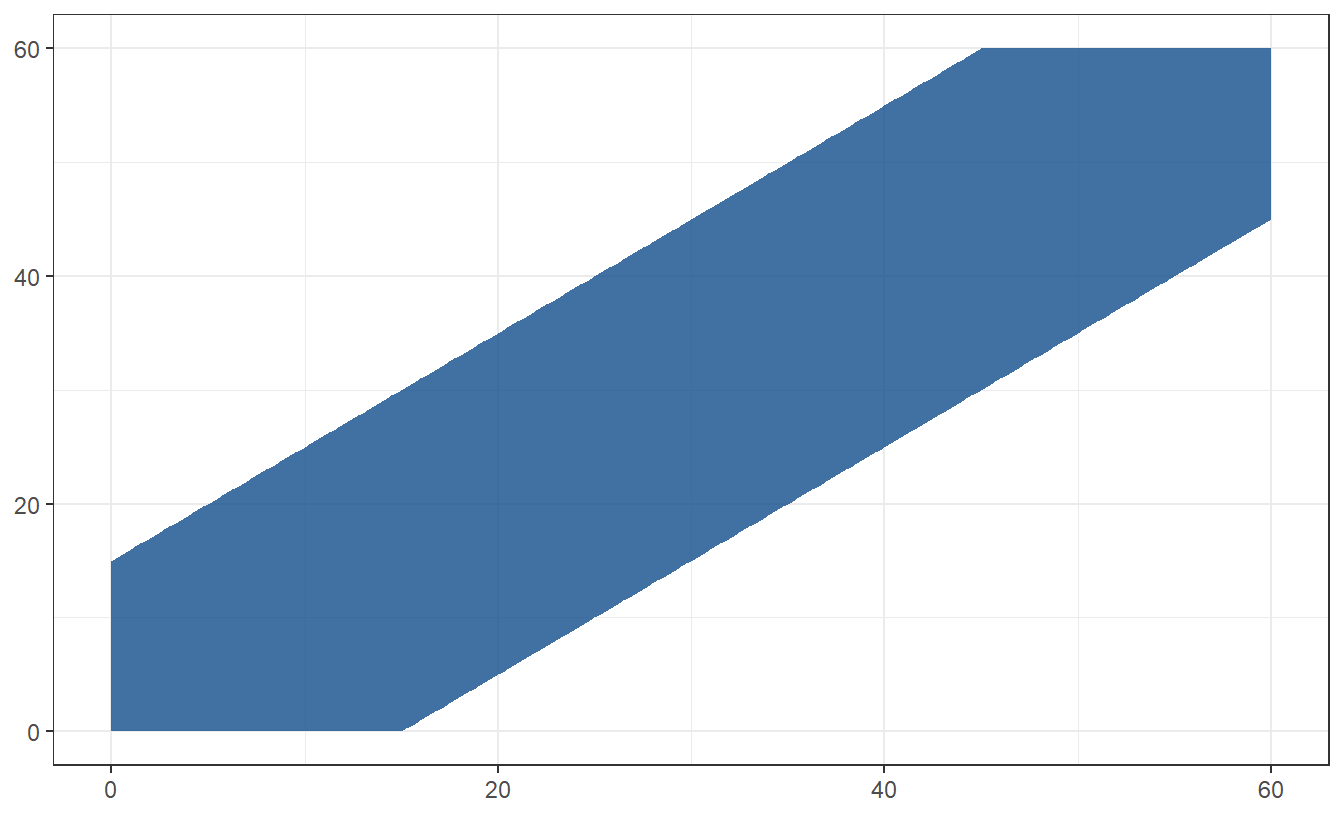
The blue area can be easily calculated to be \(\vert A \vert = 60^2-45^2 = 1575\). Consequently, the probability that Lars and I meet is given by \(\frac{1575}{3600} = 0.4375\).
Now, let us compare this probability to what we would compute using the Monte-Carlo method. Here, this would simply mean independently simulating many arrival times for Lars and I and count how many of the resulting two-dimensional random vectors fall within the blue area, i.e. which of those have arrival times differing by at most 15 minutes.
set.seed(123)
# Number of simulated arrival times
N <- 1000000

# Arrival times of Albert and Lars
A <- runif(N, min = 0, max = 60)
L <- runif(N, min = 0, max = 60)

# Count how many times the meeting can take place
c <- (abs(A - L) <= 15) %>% sum()
# Compute relative frequency
(prob <- c / N)
#> [1] 0.437475
This comes pretty close to the real result. Of course, if we increase the amount of simulated arrival times we can probably get even closer to the real probability.
Naturally, the Monte-Carlo method is not only used to confirm probabilities we can compute analytically. The real strength of the method lies in the fact that we can use it even when the involved quantities are hard to deal with analytically. Also, we may not only compute probabilities as we did before but we may compute any interesting quantity that can be expressed as expectation \(\mathbb{E}g(X)\) of some random variable \(g(X)\) which itself may be a (complicated) function of an underlying random variable \(X\).
5.1 Poisson process
In this chapter, we have only looked at independent random variables so far. Thus, the quantities we tried to compute were only dependent on the random variables’ marginal distributions. Obviously, not everything can be modeled via independent random variables which often complicates things analytically.
For instance, let us look at a stochastic process \(X = \{X(t), t \geq 0 \}\) which is nothing but a family of random variables indexed by a set \(T\) (here \(T = [0, \infty)\)). More specifically, let us look at a Poisson process \(N = \{N(t), t \geq 0 \}\) with rate \(\lambda > 0\) which is defined as a stochastic process that fulfills \[\begin{align*} N(t) = \max\bigg\{n \in \mathbb{N}\, \bigg\vert\, \sum_{k = 1}^n Y_k \leq t \bigg\} \end{align*}\] where \(Y_k\), \(k \in \mathbb{N}\), are iid. \(\text{Exp}(\lambda)\) random variables. Consequently, \(X(t_1)\) and \(X(t_2)\) are not independent as they both depend on the distribution of (multiple) \(Y_k\). A trajectory or path, i.e. a realization, of such a Poisson process may look something like this
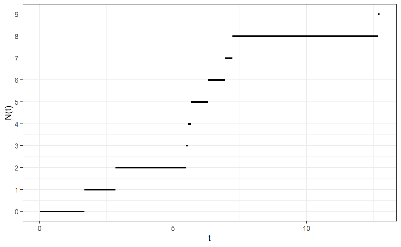
Figure 5.1: Realization of a Poisson process with rate \(\lambda = 0.5\)
Notice that simulation of such a path is straight-forward. Simply simulate independent \(\text{Exp}(\lambda)\) random variables, compute the cumulative sum of these realizations and increase \(N\) by one whenever the cumulative sum increases.
With the Monte Carlo method it is easy to compute quantities such as \(\mathbb{E}\inf\{t > 0 \vert N(t) \geq 10\}\). Since the process always jumps by at most one, we simply simulate 10 exponential random variables and compute their sum. If we do this often enough and keep denoting the sum of the realizations, we can average these times to get an approximation of \(\mathbb{E}\inf\{t > 0 \vert N(t) \geq 10\}\).
set.seed(123)
threshold <- 10    # Threshold to reach
N <- 100000        # Number of paths
lambda <- 1        # Intensity of exponential rvs

time_to_threshold <- numeric(N)
for (i in seq_along(time_to_threshold)) {
  time_to_threshold[i] <- sum(rexp(threshold, lambda))
}
# Estimate
mean(time_to_threshold)
#> [1] 9.998061
Admittedly, we could have computed this ourselves by realizing that the sum of \(n\) iid. exponential random variables follows a gamma distribution whose expected value can be easily computed to be \(n\). Nevertheless, it is good to have seen this approach as it generalizes well.
Now, imagine that instead of making unit jumps, the Poisson process can make arbitrary jumps. This kind of thinking leads us to the notion of the compound Poisson process.
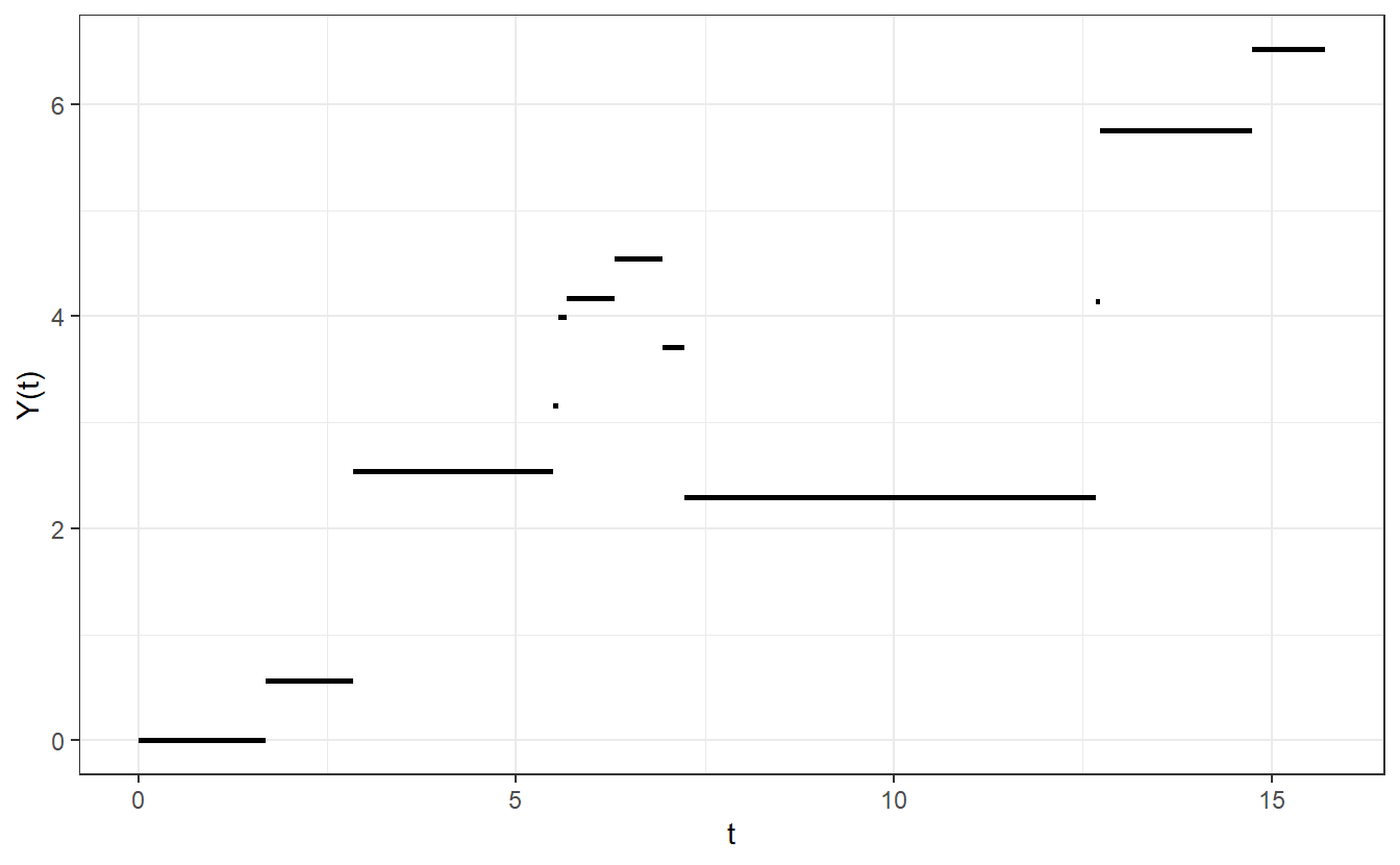
Suppose that \((\xi_n)_{n \in \mathbb{N}}\) is a sequence of iid. random variables. These will represent the jumps of the compound Poisson process. Thus, a compound Poisson process is a stochastic process \(Y = \{Y(t), t \geq 0 \}\) where \(Y(t)\) can be characterized by \[\begin{align*} Y(t) = \sum_{k = 1}^{N(t)} \xi_k \end{align*}\] where \(N = \{ N(t), t \geq 0 \}\) is a Poisson process.
If \(\xi_1 \sim \text{U}(-2, 2)\), then a path of a compound Poisson process with intensity \(\lambda = 0.5\) may look like this
Theoretically, any probabilities and expectations involving the compound Poisson process come with the additional complexity of having to know the distribution of the \(n\)-fold convolution of \(\xi_k\), \(k = 1, \ldots, n\) where \(n\) can be any arbitrary positive integer. As for simulations, the only real threshold we need to cross is that we have to be able simulate realizations from the distribution of \(\xi_1\).
In ruin theory, a part of actuarial science focusing on the possibility of an insurer’s financial ruin, compound Poisson processes are a popular tool. For instance, you may imagine that an insurer is vulnerable to claims it has to pay as part of its insurance contracts. These claims can be random in numbers and height. In return, the insurer gets a steady stream of premiums \(c > 0\) from its customers. Additionally, it may currently have a amount of cash \(c_0\).
Now, the so-called classical Cramér-Lundberg model describes the assets of an insurer over time via a stochastic process \(X = \{ X(t), t \geq 0 \}\) defined via \[\begin{align*} X(t) = c_0 + ct - \sum_{k = 1}^{N(t)} \xi_k \end{align*}\] where \(N = \{ N(t), t \geq 0 \}\) is a Poisson process with rate \(\lambda > 0\).
Naturally, one may ask what the probability is that the insurer will experience financial ruin in the next, say, 10 years, i.e. we are interested in the quantity \(\mathbb{P}(\inf\{ t \geq 0\, \vert\, X(t) < 0 \} \leq 10)\). Let us compute this quantity via the Monte Carlo method assuming that \(\xi_1 \sim \text{Exp}(\lambda_{\text{claims}})\), with \(\lambda_{\text{claims}} > 0\).
set.seed(123)
# Initial parameters
lambda_N <- 2
lambda_claims <- 3
c_0 <- 0.25
c <- 1
N <- 10000
time_horizon <- 10

# Monte Carlo simulation
ruin_occurred <- logical(N)
for (i in seq_along(ruin_occurred)) {
  t <- 0
  X <- c_0
  ruin <- FALSE
  while (t <= time_horizon) {
    waiting_time <- rexp(1, lambda_N)
    xi <- rexp(1, lambda_claims)
    t <- t + waiting_time
    X <- X + c * waiting_time - xi
    if (X < 0) {
      ruin <- TRUE
      break  # break out of while-loop
    }
  }
  ruin_occurred[i] <- ruin
}

# Estimate probability
mean(ruin_occurred)
#> [1] 0.5107
Thus, with the initial parameters that were chosen here, the insurer has approximately a 50-50 chance to go bankrupt. Of course, the initial parameters were chosen arbitrarily. In practice, an insurer will have to use its historic records to figure out what a good choice of the initial parameters is.
5.2 Brownian Motion / Wiener Process
In financial mathematics, there is an infamous market model called Black-Scholes model. In its simplest form, this model assumes that the market consists of
- one risk-free asset that delivers a constant rate of return \(r\) and
- one risky stock whose price is described by a so-called geometric Brownian motion with constant drift \(\mu\) and volatility \(\sigma\).
Let us untangle the latter asset step by step. A Brownian motion or Wiener process is a stochastic process \(W = \{W(t), t \geq 0\}\) that fulfills
- \(W(0) = 0\)
- \(W\) has continuous trajectories
- \(W\) has independent increments which implies that \(W(t + s) - W(t)\), \(s \geq 0\), is independent of the past values \(W(x)\), \(x \leq t\)
- \(W(t + s) - W(t) \sim \mathcal{N}(0, s)\) for all \(s, t \geq 0\)
The Poisson process we looked at earlier has condition 1 and 3 in common with the Brownian motion. Of course, there is a lot more to know about the Brownian motion as it is one of the best studied stochastic processes. But as we are only trying to use these type of processes for simulation purposes, let us stick to just that.
To do so, it is worth noting that from the above conditions one can deduce that for all \(0 < s < t\) it holds that \(W(t) = W(s) + \sqrt{t - s} Z\) where \(Z\) is a standard normal random variable. Combined with \(W(0) = 0\) this allows us to iteratively simulate a trajectory of a Brownian motion on a grid \(t = 0, \text{dt}, 2\text{dt}, \ldots, T\) where \(\text{dt}\) decribes the finenness of the grid. This may look like this:
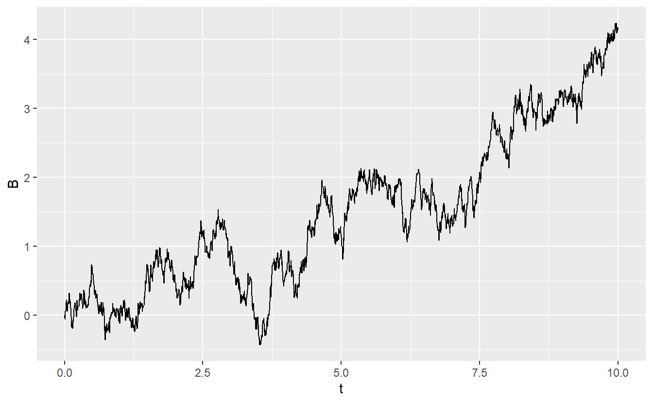
Now, a geometric Brownian motion \(S = \{ S(t), t \geq 0 \}\) with drift \(\mu\) and volatility \(\sigma\) can be computed via \[\begin{align*} S(t) = S(0) \exp \bigg\{ \bigg( \mu - \frac{\sigma^2}{2} \bigg)t + \sigma B(t) \bigg\} \end{align*}\] where \(B = \{ B(t), t \geq 0 \}\) is a Brownian motion and \(S(0)\) is some initial value of \(S\). Consequently, the above realization of a Brownian motion can be used to give the following realization of a geometric Brownian motion with drift \(\mu = 0.06\), volatility \(\sigma = 0.15\) and initial value \(S(0) = 1\).
mu <- 0.06
sigma <- 0.15
S_0 <- 1

# t is time scale of previous Brownian motion
# B is previous realization of Brownian motion
S <- S_0 * exp((mu - sigma^2 / 2) * t + sigma * B)
tibble(
  t = t,
  S = S
) %>%
  ggplot() +
  geom_line(aes(t, S))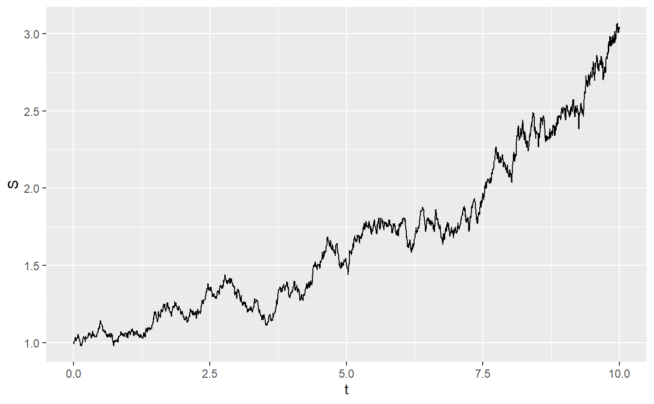
In the Black-Scholes model, this now may be considered as the stock price evolution over time. One reason why this model is so popular is that it enables us to compute the value of a so-called European call option on the stock \(S\).
A European call option is a financial contract between two parties that gives the buyer of said option the opportunity to buy a stock share at a so-called strike price \(K\) at a predetermined time \(T\) in the future.
On one hand, the buyer of a call option can make a profit if the strike price \(K\) is lower than the stock price at the time of execution, i.e. if \(K < S(T)\). On the other hand, if \(K > S(T)\) then the buyer will simply not use the option (because why would anyone pay more than necessary at the regular market). Thus, the payout of a call option at time \(T\) can be summarized as \(C = \max\{S(T) - K, 0\}\).
Of course, this begs the question: What is the value of such an option, i.e. what would be a good price to pay for such an option? In the Black-Scholes model there is a theoretical answer to this. At any time \(t \in [0, T]\) this answer depends on the
- time to maturity \(T - t\),
- current price of the risky asset \(S(t)\),
- strike price \(K\),
- volatility \(\sigma\) of the risky asset and
- the risk-free return \(r\) from the risk-free asset in the market.
Given these quantities, the Black-Scholes formula delivers the value of an European call option \(C_t\) at time \(t\) by \[\begin{align*} C_t = \Phi(d_1)S_t - \Phi(d_2) K e^{-r(T - t)}, \end{align*}\] where \(\Phi\) is the distribution function of the standard normal distribution and \[\begin{align*} d_1 &= \frac{1}{\sigma \sqrt{T - t}} \bigg[ \log \frac{S_t}{K} + \bigg( r + \frac{\sigma^2}{2} \bigg) (T - t) \bigg]\\ d_2 &= d_1 - \sigma\sqrt{T-t} \end{align*}\]
Let us use these (maybe complicated looking) formulas as a base line to determine the value of a European call option Monte Carlo-style. This can be accomplished as follows:
- Simulate a lot of paths of the risky asset (under the so-called risk-neutral measure which here simply means that \(\mu = r\))
- Compute the payoff of the option for each path
- Average the payoffs
- Since the option pays in the future we need to compute their value at time \(t\) via discounting the average by multiplying it by \(e^{-r(T-t)}\).
In order for step 1 to work, I have implemented a function generate_geom_BM(mu, sigma, S_0, time_horizon, dt = 0.025) that simulates a path from 0 to time_horizon in steps of length dt = 0.025 with parameters mu, sigma and S_0 (you will get to implement that in the exercises).
The output of said function is as follows
mu <- 0.06
sigma <- 0.15
S_0 <- 1
time_horizon <- 10
generate_geom_BM(mu, sigma, S_0, time_horizon)
#> # A tibble: 401 x 2
#>       t     S
#>   <dbl> <dbl>
#> 1 0     1
#> 2 0.025 0.989
#> 3 0.05  0.996
#> 4 0.075 0.984
#> 5 0.1   1.01
#> 6 0.125 1.02
#> # ... with 395 more rows
Now we can follow the above steps and compute the call option price at time \(t = 0\) and compare it to the theoretical value.
set.seed(123)
sigma <- 0.15
S_0 <- 1
time_horizon <- 10
r <- 0.02
K <- 1
N <- 10000

# Theoretical price
d_1 <- 1 / (sigma * sqrt(time_horizon)) * (
  log(S_0 / K) + (r + sigma^2 / 2) * time_horizon
)
d_2 <- d_1 - sigma * sqrt(time_horizon)
val_theo <- pnorm(d_1) * S_0 - pnorm(d_2) * K * exp(-r * time_horizon)

# Simulated price
payoff <- numeric(N)
for (i in seq_along(payoff)) {
  # Choose mu = r here for "risk-neutral measure"
  S <- generate_geom_BM(r, sigma, S_0, time_horizon)$S
  payoff[i] <- max(S[length(S)] - K, 0)
}
val_simu <- exp(-r * time_horizon) *  mean(payoff)

# Output
glue::glue("Theoretical value: {val_theo}")
#> Theoretical value: 0.275713492487472
glue::glue("Monte-Carlo value: {val_simu}")
#> Monte-Carlo value: 0.271898095322233
As you can see, the Monte-Carlo approach delivers a result which is very close to the theoretical result. Again, the Monte-Carlo approach is not really “necessary” here since there already is a formula to price the call option. However, Monto-Carlo option pricing is hugely popular among practitioners as it allows to price even more exotic financial derivatives when there is no analytic solution.
5.3 Exercises
5.3.1 The Poisson Process
Write a function simulate_PP(lambda, time, grid) which simulates a Poisson process with rate lambda from time zero to time on a grid with fineness grid and returns a tibble consisting of the columns t and X.
Here, t contains all grid points from zero to time and X denotes the value of the Poisson process at time t.
For instance, the result may look like this.
set.seed(1234)
simulate_PP(lambda = 0.5, time = 5, grid = 0.5)
#> # A tibble: 11 x 2
#>       t     X
#>   <dbl> <dbl>
#> 1   0       1
#> 2   0.5     1
#> 3   1       1
#> 4   1.5     1
#> 5   2       1
#> 6   2.5     1
#> # ... with 5 more rows
Use it to compute multiple box plots summarizing the distributions of \(X(n)\), \(n \in \{1, \ldots, 10\}\), where \(X\) is a Poisson process with rate \(\lambda = 1\). Also, indicate the theoretical expected value \(\mathbb{E}X(n) = n\) via a red dot. Your plots should be based on 1000 realizations of the Poisson process and should look something like this.
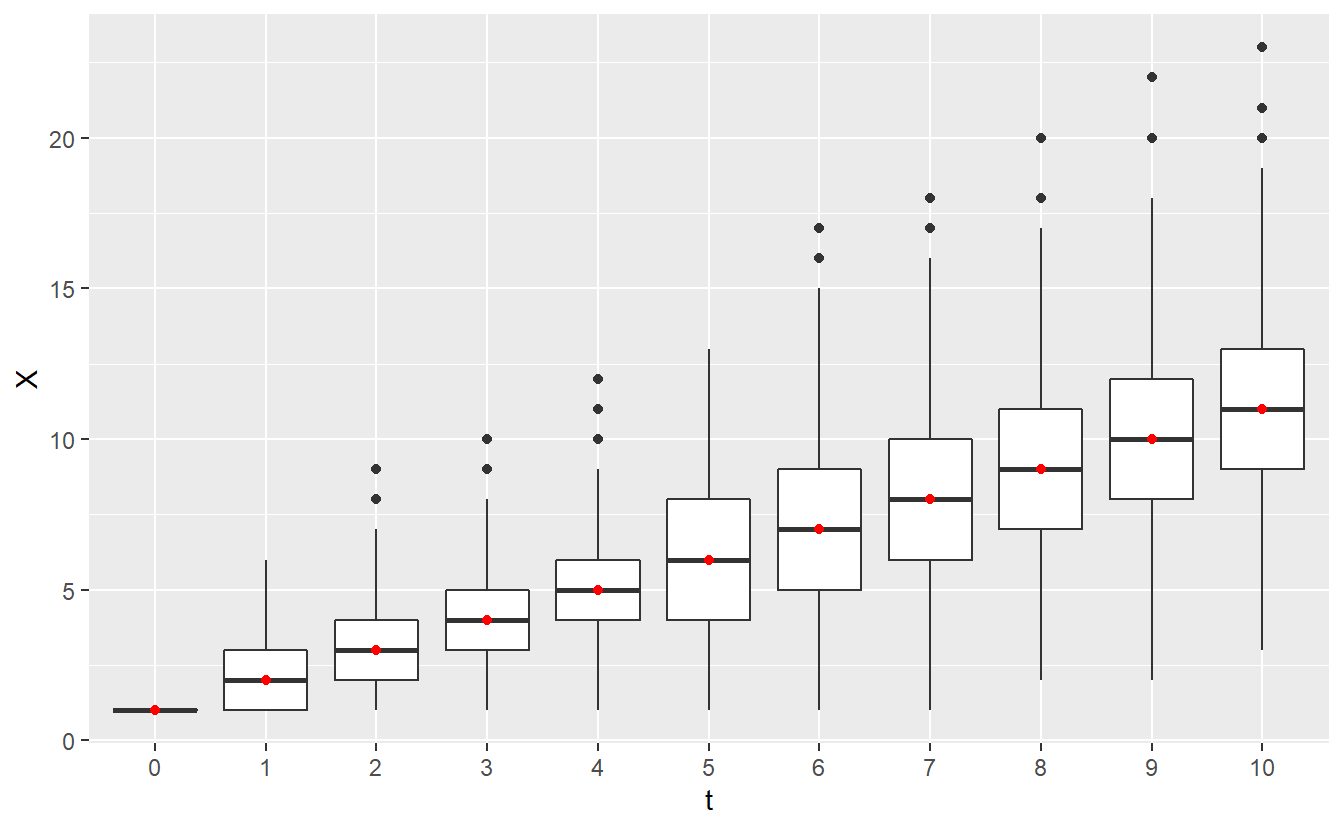
Hint: You may collect the simulated processes in a tibble via iteratively extending a tibble in a for loop. Even though this is not efficient, we have not covered lists in great detail yet which are a convenient format for such purposes. So, the slow method is fine, too.
5.3.2 Ruin Theory
Write a function estimate_ruin(lambda_N, dist, param, N) that estimates the 5-year ruin probability in the Cramér-Lundberg model with parameters \(c_0 = 10\), \(c = 2\) based on N realizations of a compound Poisson process with rate lambda_N. The variables dist and param shall be used to indicate the one-parameter distribution family of the compound Poisson process’ jumps and the value of its parameter.
Use your defined function to estimate the 5-year probabilities in the Cramér-Lundberg model with parameters \(c_0 = 10\), \(c = 2\) based on 10000 realizations of a compound Poisson process with rate 2 where the process’ jumps follow
- a geometric distribution with parameter 0.4 (the geometric distribution that R implements can be used here)
- a geometric distribution with parameter 0.25 (the geometric distribution that R implements can be used here)
- a Poisson distribution with parameter 2
- a \(\chi^2\)-distribution with 2.5 degrees of freedom
5.3.3 (Geometric) Brownian Motion
Implement the previous function generate_geom_BM(mu, sigma, S_0, time_horizon).
5.3.4 Gaussian Processes
A Gaussian process is a stochastic process \(X = \{X(t), t \in T \}\) whose finite-dimensional distributions follow a multivariate Gaussian distribution, i.e. for all indices \(t_1, \ldots, t_n \in T\), \(n \in \mathbb{N}\) it holds that the random vector \((X(t_1), \ldots, X(t_n))\) is a multivariate normal distribution with mean parameter \(\mu\) and covariance matrix \(\Sigma\).
Fundamentally, what makes Gaussian processes so popular is that they can be completely described via a mean funcion \(m(t) = \mathbb{E}X(t)\) for all time points \(t \in T\) and a covariance function \(Cov(X(t), X(t'))\) for any two time points \(t, t' \in T\).
Now, simulate a Gaussian process \(X(t)\) for \(t = 0, 0.05, 0.1, \ldots, 5\) whose mean function is given by \(m(t) = 0\) and \(Cov(X(t), X(t')) = [\exp(-\vert t - t'\vert) - \exp(-(t + t'))]/2\).
To do so, you may (without a proof) use that if you remove components of a random vector that follows a multivariate normal distribution with parameters \(\mu\) and \(\Sigma\), then the resulting vector again follows a multivariate normal with parameters \(\mu'\) and \(\Sigma'\) which are computed by removing the parameters from \(\mu\) and \(\Sigma\) that correspond to the eliminated components. See marginal distributions on Wikipedia for an example of this.
Consequently, you only have to simulate a realization from a multivariate normally distributed random vector with mean parameter zero and appropriate covariance matrix to simulate this Gaussian process.
Hint: MASS::mvrnorm() can simulate multivariate normal distributions, pracma::zeros() can generate a matrix filled with zeros and which(boolean_matrix, arr.ind = T) can return the row and column indices of entries in a boolean matrix that are TRUE.