4 Random Number Generators
In this chapter, we want to talk about randomness. Surely, if we want to extract meaning from data, we will have to differentiate between actual patterns and random fluctuations. Thus, a quick study of randomness is in order.
Of course, everything from philosophical to mathematical aspects of randomness cannot possibly be covered here. Therefore, let us focus on how to generate numbers that look convincingly random.
What do I mean by that? Imagine a scatter plot of a lot of randomly scattered points in the unit square, i.e. in \([0, 1]^2\). What you imagine may look like this.

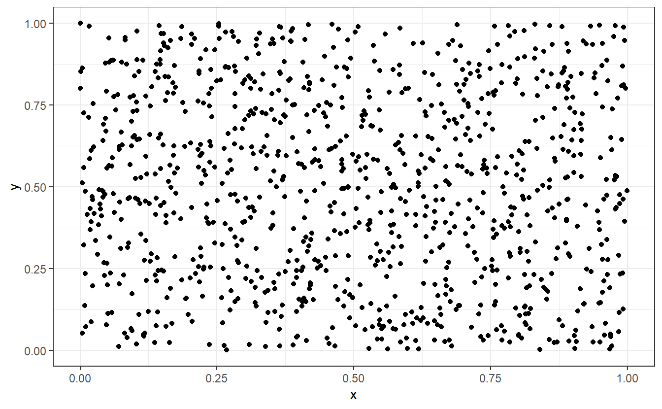
Wikipedia describes randomness as “the apparent lack of pattern or predictability in events”44 and intuitively, most people would probably say that this picture right here certainly fits that bill. However, you may (rightfully) suspect that this picture is not “truly” random in the sense that there is no definite way to recreate this picture. That is, of course, because there is a way to recreate this plot.
I simulated numbers between 0 and 1 to use as x- and y-coordinates of the points and the rest was only a matter of calling ggplot()
.
Naturally, this implies that there is a way to generate numbers that (hopefully) look the random part but are, in fact, anything but random because someone has to instruct R “what” to compute.
As we know from elementary probability classes, randomness can come in different shapes in the sense of different probability distributions. For instance, look at this new scatter plot:

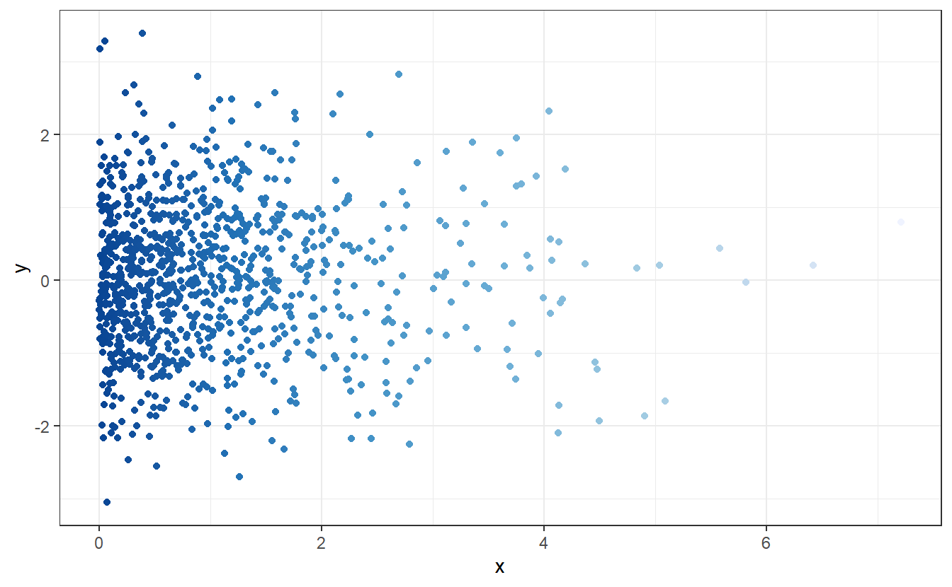
Here, the points look scattered all over the place45. This time, however, it looks like there seems to be at least some overall tendencies present. More specifically, it appears that there are way more points whose x- and y-coordinates are close to zero.
We can discern these patterns, if we look only at the x- and y-coordinates and their distribution.
Same as we did in Chapter 2, we can plot an estimation of the corresponding densities via geom_density()
.
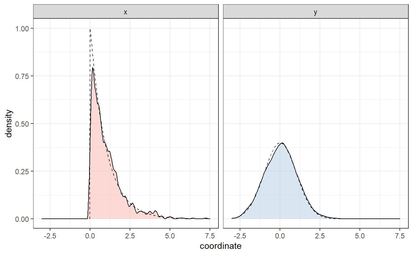
This basically resembles what we have surmised from the scatter plot: In both coordinates, values close to zero are favored way more than others. Interestingly, these estimated densities look similar to the densities of an exponential resp. a Gaussian distribution (as seen by the dashed lines). These were in fact the distributions I was aiming to simulate in the second scatter plot.
Consequently, it is also possible to generate numbers that can pass of as realizations of an exponential or Gaussian distribution. In the course of this chapter, we will see that we can do that for many more distributions.
4.1 Simulating Uniformly Distributed Random Variables
The basis for many simulation techniques is the ability to simulate numbers that appear to be uniformly distributed on \([0, 1]\). As the introduction suggests, none of the simulated numbers are “truly random” which is why they are usually called pseudorandom numbers.
One of the most basic generator of pseudorandom numbers are so-called linear congruential generators (LCG). These generate numbers on a set \(E = \{ 0, \dots, m - 1\}\) where \(m \in \mathbb{N}\) is a given positive integer. The specific recursive generation procedure for a pseudorandom number \(x_n\) is given by \[\begin{align*} x_{n+1} = (ax_n + c) \mod m, \end{align*}\] for fixed constants \(a, c \in \mathbb{N}\). Dividing these numbers by \(m\) will lead to numbers in \([0, 1]\).
Finally, the above recursion implies that we need some initial value \(x_0\). This initial value is usually called seed and is often chosen as something “random”, e.g. decimal places of the generator’s starting time.
Note that the knowledge of the generator, i.e. the above recursion formula and the constants \(a, c\) and \(m\), make the pseudorandom numbers reproducible. Reproducibility can be of advantage if you are working with simulations so that other researches/coworkers can reproduce your findings. Also, it helps to compare for instance two procedures on the same pseudorandom numbers. Otherwise, you may never know if differences in the procedures are due to random fluctuations or a different performance of either procedure.
Let us implement a LCG with some initial parameters. To do so, we will have to learn about for-loops. Theses help us for sequential computations such as the above recursion. The general syntax of R’s for-loop looks like this
for (<loop index> in <loop range>) {
<instructions here>
}
In our case, this may look like this
# Coefficients of LCG
m <- 100
a <- 4
c <- 1
seed <- 5
# Create empty vector so that we can fill it with
# pseudorandom numbers
n <- 15
x <- numeric(n)
x[1] <- seed
# Loop through recursion
for (i in 1:(n-1)) {
x[i + 1] <- (a * x[i] + c) %% m
}
x
#> [1] 5 21 85 41 65 61 45 81 25 1 5 21 85 41 65
Dividing x
by m
would then lead to the desired numbers on \([0, 1]\).
However, if you look at the sequence of numbers you may notice that there is evil afoot46.
Obviously, there is some periodicity to the numbers which will not help us on our pursuit of randomness.
This periodicity may be eleviated by a “better” choice of the LCG parameters. One such choice leads to so called RANDU generator.
# RANDU coefficients
m <- 2^31
a <- 65539
c <- 0
seed <- 1 # any odd positive integer
# Create empty vector so that we can fill it with
# pseudorandom numbers
n <- 16
x <- numeric(n)
x[1] <- seed
# Loop through recursion
for (i in 1:(n-1)) {
x[i + 1] <- (a * x[i] + c) %% m
}
x
#> [1] 1 65539 393225 1769499 7077969 26542323
#> [7] 95552217 334432395 1146624417 1722371299 14608041 1766175739
#> [13] 1875647473 1800754131 366148473 1022489195
Figure 4.1: Scatter plot of \((x_k, x_{k + 1}, x_{k + 2})\) where \(x_k\) are the 100000 realisations of the RANDU LCG (see also Wikipedia)
As you can see (go ahead, touch the interactive plot, you can rotate the plot), the points are all distributed on parallel planes. This does not foster great confidence in the numbers’ randomness. Consequently, LCGs are discouraged to use though they serve nicely as an introduction into how generation of random numbers can be thought about.
R and many other programming language use something called Mersenne Twister.
We do not really have to think about what this generator does but it suffices to say that it has less drawbacks than LCGs.
In R, we can employ it using runif()
(as in “realisations of uniformly distributed random variables”).
For reproducibility, its seed can be fixed via set.seed()
.
4.2 Simulating General Random Variables
By now, we are able to draw (simulate) samples from a continuous uniform distribution on \([0, 1]\), i.e. realizations from a random variable \(X \sim U(0, 1)\). Generally, we aim at transforming these samples such that they can be thought of as a sample from a different distribution.
For instance, one very simple example uses the fact that \(aX + b \sim U(b, a + b)\) if \(X \sim U(0, 1)\) for \(a \neq 0\) and \(b \in \mathbb{R}\). Consequently, we may draw a sample \(x\) from \(U(0, 1)\) and transform it by \(y = ax + b\) such that we can think of \(y\) as a sample from \(U(a,a+b)\). Let’s see if that holds true empirically.
a <- 2
b <- 1
set.seed(12345)
tibble(
x = runif(100000),
y = a * x + b
) %>%
ggplot() +
geom_histogram(aes(y, y = ..density..)) +
coord_cartesian(xlim = c(0.5, 3.5))
#> `stat_bin()` using `bins = 30`. Pick better value with `binwidth`.

This looks the way a histogram of a \(U(1, 1 + 2)\)-sample should look like. Thus, it is possible to generate other uniform samples through a linear transformation of a standard-uniform sample.
The so-called inversion method will allow us to use other than linear transformations to generate samples from other distribution families. Finally, the acceptance-rejection method will use samples from both a uniform and non-uniform distribution to generate a sample from a third distribution.
4.2.1 Inversion Method
Suppose \(X\) is a random variable with distribution function \(F_X\). Then, the distribution’s quantile function is defined as the generalized inverse \(F_X^{\leftarrow}\) of \(F_X\) where \(F_X^{\leftarrow}\) is defined as \[\begin{align*} F_X^{\leftarrow}(u) = \inf \{ x \in \mathbb{R}\, \vert\, F_X(x) \geq u \} \end{align*}\] for all \(u \in [0, 1)\).
The inversion method relies on the fact that the random variable \(F_X^{\leftarrow}(U)\), where \(U \sim\) \(U(0, 1)\), has distribution function \(F_X\), i.e. follows the same distribution as \(X\). Consequently, we have found a method that justifies the following algorithm:
- Compute quantile function \(F_X^{\leftarrow}\) of desired distribution
- Draw sample \(u\) from standard-uniform distribution
- \(x = F_X^{\leftarrow}(u)\) can now be thought of as a sample from distribution of \(X\)
Example 4.1 Let us draw samples from an exponential distribution \(\text{Exp}(\lambda)\) with parameter \(\lambda > 0\). Its distribution function is given by \[\begin{align*} F(x) = 1 - e^{-\lambda x} \end{align*}\] for all \(x \geq 0\) and \(F(x) = 0\) otherwise.
Now, elementary computations lead to \[\begin{align*} F^{\leftarrow}(u) = - \frac{\log (1- u)}{\lambda} \end{align*}\] for all \(u \in [0, 1]\).This can be easily simulated. Let us do that and compare the corresponding histogram to the theoretical density. For the histogram we will have to adjust the default’s binwidth in order to catch the behavior close to zero better.
set.seed(123)
lambda <- 2
simu_data <- tibble(
u = runif(100000),
x = -log(1 - u) / lambda
)
density_data <- tibble(
t = seq(0.01, max(simu_data$x), 0.01),
density = dexp(t, rate = lambda) # density of exponential
)
simu_data %>%
ggplot() +
geom_histogram(aes(x, y = ..density..), binwidth = 0.01) +
geom_line(data = density_data, aes(t, density), col = "red")

Similarly, we can also simulate realizations from discrete random variables.
Again let us use this and compare the histogram to the real distribution.
set.seed(123)
p <- 0.3
density_data <- tibble(
x = c(0, 1),
y = c(1- p, p)
)
tibble(
u = runif(100000),
x = between(u, 1-p, 1) * 1 # * 1 converts logical to double
) %>%
ggplot() +
geom_bar(aes(x, y = ..prop..)) +
geom_point(
data = density_data,
aes(x, y),
col = "red",
size = 2
)

4.2.2 Acceptance-Rejection Method
Imagine that you use the previous methods to simulate independent realizations \(u_i, x_i\), \(i = 1, \dots, N\), \(N \in \mathbb{N}\), of the random variables \(U \sim U(0,1)\) and \(X \sim \text{Exp}(\lambda)\), \(\lambda > 0\), respectively.
Imagine further that you now use these realisations to plot the points \((x_i, u_i f_X(x_i))\) and \(f_X\), where \(f_X\) is the density of \(X\).
This may look like this.
As you can see, these these points fill up the area between the x-axis and the density function of \(X\). What you may not see immediately but what is true if you think about it, is the fact that the amount of points for a given value of \(x\) is related to \(f(x)\). Obviously, this comes from the fact that we simulated realisations \(x_i\) of \(X\).
Similarly, if we scale the y-coordinates of the points by a factor \(k > 1\), i.e. plot \((x_i, k u_i f_X(x_i))\), then the points will fill the area under \(kf_X(x)\). Thus, we could use this fact to generate realizations of a different random variable \(Y\) whose density \(f_Y\) we can bound from above by \(kf_X\). We do this by filling the area under \(kf_X\) with the help of realizations of \(X\) as above but rejecting points that do not also fall within the area under \(f_Y\). We check the latter by checking whether \(\frac{k u_i f_X(x_i)}{f_Y(x_i)} < 1\). This procedure is known as acceptance-rejection method.
Imagine that we want to simulate a random variable \(Y\) that follows a Gamma distribution with parameters 3/2 and 1, i.e. \[\begin{align*} f_Y(y) = \frac{2}{\sqrt{\pi}} \sqrt{y} e^{-y} \end{align*}\] for \(y > 0\).
We will use the density \(f_X\) of an \(\text{Exp}(2/3)\) random variable to bound \(f_Y\) from above. To do so, we will need to find a constant \(k\) such that \(f_Y < kf_X\) by finding the maximum of \(h(x) = f_Y(x)/f_X(x)\). Through elementary calculus it can be seen that \(h\) is maximal for \(x = 3/2\) which gives us \[\begin{align*} k = h(3/2) = 3 \sqrt{\frac{3}{2 \pi}} e^{-1/2}. \end{align*}\] Thus the desired density and the rejection area look like so:
Figure 4.2: Density of Gamma distribution (in green) and rejection area (in red)
Now, to implement the acceptance-rejection method, we will have to use if-conditions to check whether a simulated point is in the rejection area. In R, the general structure of if-conditions is given as follows
if (<condition>) {
<statement if condition is true>
else {
} <statement if condition is false>
}
For short if-conditions and corresponding statements R allows it to write everything in one line. Personally, I dislike that style but it may be worth noting this style of writing is possible if you so desire. Further, we will need while-loops to keep generating random variables until we can accept one. In R, the general structure of while-loops is given as follows
while (<condition>) {
<statement while condition is true>
}
Here, we will use while
and if
in conjunction to loop until we can accept a realization and then set the looping condition to FALSE
.
set.seed(123)
lambda <- 2 / 3
k <- 3 * sqrt(3 / (2 * pi)) * exp(-1/ 2)
# Boolean for rejection, initial state needs to be TRUE
rejected <- TRUE
while (rejected) {
# Inversion method for Exp(2 / 3) realization
u <- runif(1)
x <- -log(1 - u) / (lambda)
# independent realization of x
u <- runif(1)
# Check whether accepted or rejected
f_X <- lambda * exp(- lambda * x)
f_Y <- 2 / sqrt(pi) * sqrt(x) * exp(-x)
if (k * u * f_X / f_Y < 1) {
# Accepted so set rejected to FALSE
rejected <- FALSE
}
}
x
#> [1] 0.5086263
Similarly, we can simulate a lot of realizations:
set.seed(123)
N <- 10000
xs <- numeric(N)
for (i in seq_along(xs)) {
# Boolean for rejection, initial state needs to be TRUE
rejected <- TRUE
while (rejected) {
# Inversion method for Exp(2 / 3) realization
u <- runif(1)
x <- -log(1 - u) / (lambda)
# independent realization of x
u <- runif(1)
# Check whether accepted or rejected
f_X <- lambda * exp(- lambda * x)
f_Y <- 2 / sqrt(pi) * sqrt(x) * exp(-x)
if (k * u * f_X / f_Y < 1) {
# Accepted so set rejected to FALSE
rejected <- FALSE
}
}
xs[i] <- x
}
# See if realizations look like gamma density
x <- seq(0, max(xs), 0.05)
f_Y <- 2 / sqrt(pi) * sqrt(x) * exp(-x)
ggplot() +
geom_histogram(aes(x = xs, y = ..density..), binwidth = 0.1) +
geom_line(aes(x, f_Y), col = "red", size = 1) +
theme_bw()

This looks pretty decent. So, we can assume that the acceptance-rejection method delivered the results we were wishing for.
However, notice that depending on what density \(f_X\) and constant \(k\) we use to bound the density \(f_Y\),it can take a lot of trials before we can accept one realization. For instance, imagine that in our previous example we would have used a larger value \(k\). Immediately, this would lead to a larger rejection area in Figure 4.2.
Therefore, a good choice of \(k\) and \(f_X\) is crucial for the efficiency of the acceptance-rejection method. Here, however, we did not have any other means to simulate the realizations from the gamma distribution as we do not have a closed form of the quantile function. Another popular distribution for which this is the case is the normal distribution which we want to talk about next.
4.2.4 R Commands
Naturally, R already comes with routines to simulate the most common distributions. So while it is interesting to learn how simulations can be implemented, often we can use R’s own procedures. Except, of course, in the exercises of this chapter. There, you will have to generate realizations from certain distributions yourself.
Nevertheless, let us briefly talk about R’s simulation procedures here.
All of R’s simulation start with r
(for realization) followed by the distribution’s abbreviation, e.g. runif()
, rexp()
, rbinom()
, rnorm()
, etc.
To find out how to adjust the parameters of a specific distribution, e.g. \(\lambda > 0\) of \(\text{Exp}(\lambda)\), you will have to look into the function’s documentation.
What you will find out, if you do so, is that on the documentation page there are multiple functions described.
In fact, for each distribution R has not only a function with r
prefix but it also uses the prefixes q
(for quantile), d
(for density) and p
(for probability meaning the distribution function).
Sometimes you will have to be careful with R’s own functions though. That is because some distributions such as e.g. the exponential, gamma or geometric distribution are defined with different parameterization in the literature.
For instance, in the case of a random variable \(X\) following a geometric distribution with parameter \(p \in (0, 1)\), there are two options. \[\begin{align*} \mathbb{P}(X = k) &= p(1-p)^k, \quad k = 0, 1, \dots\\ \mathbb{P}(X = k) &= p(1-p)^{k-1}, \quad k = 1, 2, \dots\\ \end{align*}\] Thus, you will have to check the documentation if the command you want to use really refers to the distribution you want to simulate.
4.3 Exercises
4.3.1 For-loops and if-conditions
- Use a for-loop to print all numbers between 1 and 100 that are not divisible by 3 and 4.
- Do the same thing without a for-loop. Hint: A vector consisting of TRUEs and/or FALSEs can be used as indices to access a vector’s elements. The numbers also do not have to be printed on separate lines
4.3.2 Efficiency of Vector Creation
4.3.2.1 Time measurements with tictoc
Use the functions tic()
and toc()
from the package tictoc
to measure the time it takes to create a vector of length \(N = 10{,}000{,}000\) when
- you create an empty vector
x
of length \(N\) and fill each entry ofx
via a for-loop with a number, say 3. - you initialize only the first value of the vector by
x <- 3
and iteratively extend the vector in each step of a for-loop until it has length \(N\). (Hint: Ifx
is a numeric vector of length 1, you can define, say, the second component viax[2] <- 3
and so on)
What approach is faster?
4.3.2.2 Time measurements with microbenchmark
Use microbenchmark()
from the microbenchmark
package to do the same thing.
This time use \(N = 1{,}000{,}000\).
Why does the microbenchmark()
test take longer overall?
Which time estimation is more “reliable”?
tictoc or microbenchmark?
Hint: Microbenchmark allows it to measure the time of multiple operations by bundling them together in curly brackets {
and }
.
4.3.3 Binomial distribution
Write a function my_binomial(n, size, prob)
that generates n
realizations from a binomial distribution with size size
and probability prob
.
Use it to simulate 100000 realizations of a binomial distribution with parameters \(10\) and \(0.4\) and plot a histogram based on these realizations together with the theoretical probabilities.
You may only use the runif()
for simulating realizations of random variables but you may use dbinom()
and pbinom()
to compute probabilities.
Hint: You may have to tweak the histogram options to get the result you expect.
4.3.4 Geometric Distribution
Write a function my_geom(n, prob)
that generates n
realizations from a geometric distribution with probability prob
.
In this exercise, the density of the geometric distribution is defined as
\[\begin{align*}
\mathbb{P}(X = k) &= p(1-p)^{k-1}, \quad k = 1, 2, \dots,
\end{align*}\]
where \(p\) is the probability of success.
Use my_geom()
to simulate 1000 realizations of a geometric distribution with parameter \(0.4\) and plot the empirical distribution function of your sample against the theoretical distribution function.
Here, you may use rgeom()
but you need to make sure that your realizations correspond to the above density.
Also, the function ecdf()
may be helpful.
4.3.5 Cauchy Distribution
Write a function my_Cauchy(n, location, scale)
that generates n
realizations from a Cauchy distribution with location parameter location
and scale parameter scale
.
For information on the Cauchy distribution refer to Wikipedia.
Use your function to simulate 100000 realizations of a Cauchy distribution with location 2 and scale 5 and plot an estimate of the density based on your simulated sample against the theoretical density.
You may use dcauchy()
and runif()
but not rcauchy()
here.
Hint: It is possible to transform a standard uniform variable into a standard Cauchy variable (location 0 and scale 1). Also, a standard Cauchy variable can be transformed to an arbitrary Cauchy distribution.
Hint 2: You may have to filter out realizations that are extremely large in order to estimate the density nicely with geom_density()
.
Here it could be useful to stick to the window \([-50, 50]\).
4.3.6 Normal distribution
Write a function my_Gaussian(n, mu, sigma)
that based on an acceptance-rejection method and the standard Cauchy density generates n
realizations from a Gaussian distribution with location parameter mu
and scale parameter sigma
.
Note that it is enough to generate standard Gaussian random realizations via acceptance-rejection and then transform those realizations accordingly. Further, the parameter \(k\) of the acceptance-rejection method does not have to be computed explicitly. You can simply compare the densities visually and choose a \(k\) that fits.
Use your function to generate 100000 realizations of a Gaussian random variable with mean 5 and standard deviation 2 and recreate the following plot.
Hint: The package patchwork
may help with arranging the plots.

