8 Multiple Linear Models via Maps
In Chapter 2 we looked at the life expectancies over time of a couple of selected countries using data from the gapminder package.
What’s more is that we used geom_smooth() to generate a straight line for each of these countries which then looked like this.
library(tidyverse)
country_filter <- c(
  "Germany",
  "Australia",
  "United States",
  "Afghanistan",
  "Bangladesh"
)

(selectedCountries <- gapminder::gapminder%>%
  filter(country %in% country_filter))
#> # A tibble: 60 x 6
#>   country     continent  year lifeExp      pop gdpPercap
#>   <fct>       <fct>     <int>   <dbl>    <int>     <dbl>
#> 1 Afghanistan Asia       1952    28.8  8425333      779.
#> 2 Afghanistan Asia       1957    30.3  9240934      821.
#> 3 Afghanistan Asia       1962    32.0 10267083      853.
#> 4 Afghanistan Asia       1967    34.0 11537966      836.
#> 5 Afghanistan Asia       1972    36.1 13079460      740.
#> 6 Afghanistan Asia       1977    38.4 14880372      786.
#> # ... with 54 more rows

selectedCountries %>%
  ggplot(aes(year, lifeExp, col = country)) +
  geom_point() +
  geom_smooth(se = F, method = "lm")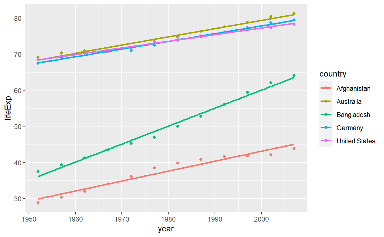
In effect, we have fitted a linear model lm(lifeExp ~ year) for each country with the help of geom_smooth().
Unfortunately, we are only left with the above picture but lack the output of lm().
Thus, for thorough analyses we will need to call lm() ourselves.
Rudimentarily, we could use a for-loop in conjunction with filter() to extract the relevant data for each country and use that to call lm().
# Only use two countries to avoid full output
for (i_country in country_filter[1:2]) {
  selectedCountries %>%
    filter(country == i_country) %>%
    lm(data = ., lifeExp ~ year) %>%
    print() # Print to force output in for-loop
}
#>
#> Call:
#> lm(formula = lifeExp ~ year, data = .)
#>
#> Coefficients:
#> (Intercept)         year
#>   -349.5415       0.2137
#>
#>
#> Call:
#> lm(formula = lifeExp ~ year, data = .)
#>
#> Coefficients:
#> (Intercept)         year
#>   -376.1163       0.2277
Here, what we’re left with is only text output of the lm() call.
However, by now we should know that lm() not only returns the estimated parameters but bundles a whole lot more information into a list.
So, it would be good if we could save these lists.
Fortunately, lists as opposed to vectors can be nested68.
nested_list <- list(
  a = "Wurst",
  b = list(c("oder", "Käse"), "Kääääse oder Wurst")
)
str(nested_list)
#> List of 2
#>  $ a: chr "Wurst"
#>  $ b:List of 2
#>   ..$ : chr [1:2] "oder" "Käse"
#>   ..$ : chr "Kääääse oder Wurst"
Thus, all we need to save the outputs of lm() is another list.
lm_list <- list()

for (i_country in country_filter) {
  lm_list[[i_country]] <- selectedCountries %>%
    filter(country == i_country) %>%
    lm(data = ., lifeExp ~ year)
}
names(lm_list)
#> [1] "Germany"       "Australia"     "United States" "Afghanistan"
#> [5] "Bangladesh"
Now, through moving along the list of lists structure via repetitive use of $ we can easily access, say, the residuals of the linear model we fitted for e.g. Afghanistan.
lm_list$Afghanistan$residuals
#>           1           2           3           4           5           6
#> -1.10629487 -0.95193823 -0.66358159 -0.01722494  0.67413170  1.64748834
#>           7           8           9          10          11          12
#>  1.68684499  1.27820163  0.75355828 -0.53408508 -1.54472844 -1.22237179
Again, this shows that a list is quite flexible so that we can use it to bundle a lot of different types of information together which is why lists are ubiquitous in R.
In fact, we have been using lists even way before we encountered lm() because a tibble is nothing other than a list.
tibble(a = "123", b = 123) %>% is.list()
#> [1] TRUE
Of course, this makes sense if you think about it because each column of a tibble is a vector where each column may consist of different data types.
Therefore, we do need a list to handle these.
What’s more is that this allows us to collect our lm() outputs within a single tibble which are - as we know - convenient to work with.
tibble(country = country_filter, linMod = lm_list)
#> # A tibble: 5 x 2
#>   country       linMod
#>   <chr>         <named list>
#> 1 Germany       <lm>
#> 2 Australia     <lm>
#> 3 United States <lm>
#> 4 Afghanistan   <lm>
#> 5 Bangladesh    <lm>
Notice that the column linmod is a column of type list.
These kind of columns are often referred to as list-like columns and are as flexible as lists.
In fact, we can even aggregate our initial data for each country in a single row like so.
nestminder <- selectedCountries %>%
  group_by(country) %>%
  nest()
nestminder
#> # A tibble: 5 x 2
#> # Groups:   country [5]
#>   country       data
#>   <fct>         <list>
#> 1 Afghanistan   <tibble [12 x 5]>
#> 2 Australia     <tibble [12 x 5]>
#> 3 Bangladesh    <tibble [12 x 5]>
#> 4 Germany       <tibble [12 x 5]>
#> 5 United States <tibble [12 x 5]>
Further, we can also collect our initial data and our model within a single tibble. Though, we will have to convert our list to a tibble first.
nestminder <- tibble(linMod = lm_list) %>%
  bind_cols(nestminder, .)
nestminder
#> # A tibble: 5 x 3
#> # Groups:   country [5]
#>   country       data              linMod
#>   <fct>         <list>            <named list>
#> 1 Afghanistan   <tibble [12 x 5]> <lm>
#> 2 Australia     <tibble [12 x 5]> <lm>
#> 3 Bangladesh    <tibble [12 x 5]> <lm>
#> 4 Germany       <tibble [12 x 5]> <lm>
#> 5 United States <tibble [12 x 5]> <lm>
Now, a relevant question may be whose country’s life expectancy on average rose the most over time, i.e. which linear model has the highest slope?
As before, we could use a for-loop to call the functions coefficients() for each row in the linMod column to extract the estimated slope of each model and bind these slopes into our nestminder tibble.
However, you may sense that this is quite tedious and requires a lot of code.
Thankfully, as we can now see, we only have to manipulate a tibble and compute a new column from existing ones.
For non-list-like columns we already learned to do this via mutate().
Luckily, the tidyverse equips us with the purrr package that comes with so-called map functions69 which allow us to handle lists somewhat effortlessly.
Combined with mutate(), map functions become powerful tools to handle list-like columns.
Therefore, we will use this chapter to explore these map functions in detail. In a way, this enhances our R skill set profoundly as it allows us to automate repetitive tasks with a lot less code than we would need using for-loops instead. Consequently, these enhanced automation skills make it easier to dive into data and may help us with the programming aspect of data analysis.
Naturally, these new skills come at a price because lists and map functions may feel quite complicated at first encounter. Though map functions could have made some tasks easier, their complexity are the reason why we avoided them so far.
(Un-)Fortunately, play time is over now, so you may now marvel at how we can run the whole previous calculations (and more) in a single pipe. Do not worry, if you do not understand the code yet, at the end of this chapter you (hopefully) will.
gapminder::gapminder %>%
  filter(country %in% country_filter) %>%
  group_by(country) %>%
  nest() %>%
  mutate(
    linMod = map(data, ~lm(data = ., lifeExp ~ year)),
    coeffs = map(linMod, coefficients),
    slope = map_dbl(coeffs, 2)
  )
#> # A tibble: 5 x 5
#> # Groups:   country [5]
#>   country       data              linMod coeffs    slope
#>   <fct>         <list>            <list> <list>    <dbl>
#> 1 Afghanistan   <tibble [12 x 5]> <lm>   <dbl [2]> 0.275
#> 2 Australia     <tibble [12 x 5]> <lm>   <dbl [2]> 0.228
#> 3 Bangladesh    <tibble [12 x 5]> <lm>   <dbl [2]> 0.498
#> 4 Germany       <tibble [12 x 5]> <lm>   <dbl [2]> 0.214
#> 5 United States <tibble [12 x 5]> <lm>   <dbl [2]> 0.184
Also, let me stress again that map() functions have one “advantage” over for-loops in the sense that they are compressed in fewer lines of code.
Here, the interplay of tibbles, mutate and map() functions allowed us to do our whole data analysis within one tibble.
Thus, we were simultaneously keeping track of intermediate results (when we want that) and collected everything in one place. Of course, all of that is possible with for-loops too but the resulting code often ends up being less concise.
8.1 Map over single input
Recall the following example from Chapter 3 where we demonstrated the principle of vectorized calculations as opposed to sequentially evaluating each row.
tib <- tribble(
  ~a, ~b,
  1, 3,
  2, 4,
  3, 5
) %>%
  mutate(minimum = min(a, b))
tib
#> # A tibble: 3 x 3
#>       a     b minimum
#>   <dbl> <dbl>   <dbl>
#> 1     1     3       1
#> 2     2     4       1
#> 3     3     5       1
Here, the minimum column is not the result of sequentially evaluating the min() function with two values from a and b which are in the same row.
This “problem” is not mutate() specific but will occur with any vectorized function.
Imagine that we want to sequentially compute the minimum of values from a and 2.
Notice that what we want to do in this example is to pass each value of column a to the following function.
Of course, using the whole column a as input for min_fct() will lead to vectorized calculation again such that the function only returns a single value.
min_fct(tib$a)
#> [1] 1
So what we could do, as before, is to write a for-loop to go through each element in column a.
More elegantly, we can map over a using the function map() from the purrr package.
This function uses the input values .x and function .f to sequentially evaluate the function at the designated input values.
map(.x = tib$a, .f = min_fct)
#> [[1]]
#> [1] 1
#>
#> [[2]]
#> [1] 2
#>
#> [[3]]
#> [1] 2
Although this returned a list instead of an vector, this at least gave the results we were looking for.
Thankfully, map() comes not alone but with brothers and sisters relating to different outputs.
Therefore, if the intended output format is clear, it is possible to use one of the following functions which use the exact same syntax as map():
-
map_dbl: Returns adoublevector -
map_chr: Returns acharactervector -
map_dfrormap_dfc: Returns a data frame created by row-binding and column-binding respectively
There are more map_*() functions which you can find in the documentation.
For our purposes, though, these will suffice.
In this example, we could have used
map_dbl(.x = tib$a, .f = min_fct)
#> [1] 1 2 2
As already mentioned, we can also use map_* in conjunction with mutate() which allows us to use a column name without $.
tib %>%
  select(a) %>%
  mutate(minimum = map_dbl(a, min_fct))
#> # A tibble: 3 x 2
#>       a minimum
#>   <dbl>   <dbl>
#> 1     1       1
#> 2     2       2
#> 3     3       2
Often, it is inconvenient to specifically define a function only so that we can use it within map().
This is especially true for simple functions as we have used in this example.
Therefore, map() allows us to define an anonymous function (anonymous since it will not have a name) via a formula using ~ in conjunction with . as placeholder for the function’s argument.
In our example this looks like this:
tib %>%
  select(a) %>%
  mutate(minimum = map_dbl(a, ~min(., 2)))
Of course, this works also for more “complex” functions.
For instance, in the introduction of this chapter I used an anonymous function to use different input as data for lm() but the formula was the same for each country.
gapminder::gapminder %>%
  filter(country %in% country_filter) %>%
  group_by(country) %>%
  nest() %>%
  mutate(
    linMod = map(data, ~lm(data = ., lifeExp ~ year))
  )
#> # A tibble: 5 x 3
#> # Groups:   country [5]
#>   country       data              linMod
#>   <fct>         <list>            <list>
#> 1 Afghanistan   <tibble [12 x 5]> <lm>
#> 2 Australia     <tibble [12 x 5]> <lm>
#> 3 Bangladesh    <tibble [12 x 5]> <lm>
#> 4 Germany       <tibble [12 x 5]> <lm>
#> 5 United States <tibble [12 x 5]> <lm>
Notice that I could not have used any function of the form map_*() here because the return object of the function lm() is a list, so I will need a list-like column.
Similarly, in the next step, I can use the coefficients() functions to extract the coefficient of each model in linMod.
But each function call will return a double vector of length greater than 1 , so again I will need a list-like column.
tib_coeffs <- gapminder::gapminder %>%
  filter(country %in% country_filter) %>%
  group_by(country) %>%
  nest() %>%
  mutate(
    linMod = map(data, ~lm(data = ., lifeExp ~ year)),
    coeffs = map(linMod, coefficients)
  )
tib_coeffs
#> # A tibble: 5 x 4
#> # Groups:   country [5]
#>   country       data              linMod coeffs
#>   <fct>         <list>            <list> <list>
#> 1 Afghanistan   <tibble [12 x 5]> <lm>   <dbl [2]>
#> 2 Australia     <tibble [12 x 5]> <lm>   <dbl [2]>
#> 3 Bangladesh    <tibble [12 x 5]> <lm>   <dbl [2]>
#> 4 Germany       <tibble [12 x 5]> <lm>   <dbl [2]>
#> 5 United States <tibble [12 x 5]> <lm>   <dbl [2]>
Finally, I can unnest the coeffs column to extract the slope coefficient from coeffs.
tib_coeffs %>%
  unnest(cols = coeffs)
#> # A tibble: 10 x 4
#> # Groups:   country [5]
#>   country     data              linMod   coeffs
#>   <fct>       <list>            <list>    <dbl>
#> 1 Afghanistan <tibble [12 x 5]> <lm>   -508.
#> 2 Afghanistan <tibble [12 x 5]> <lm>      0.275
#> 3 Australia   <tibble [12 x 5]> <lm>   -376.
#> 4 Australia   <tibble [12 x 5]> <lm>      0.228
#> 5 Bangladesh  <tibble [12 x 5]> <lm>   -936.
#> 6 Bangladesh  <tibble [12 x 5]> <lm>      0.498
#> # ... with 4 more rows
Alternatively, I can call map_dbl() to extract the second element from the coefficient vector if I am only interested in the slopes.
tib_coeffs %>%
  mutate(slope = map_dbl(coeffs, ~.[2]))
#> # A tibble: 5 x 5
#> # Groups:   country [5]
#>   country       data              linMod coeffs    slope
#>   <fct>         <list>            <list> <list>    <dbl>
#> 1 Afghanistan   <tibble [12 x 5]> <lm>   <dbl [2]> 0.275
#> 2 Australia     <tibble [12 x 5]> <lm>   <dbl [2]> 0.228
#> 3 Bangladesh    <tibble [12 x 5]> <lm>   <dbl [2]> 0.498
#> 4 Germany       <tibble [12 x 5]> <lm>   <dbl [2]> 0.214
#> 5 United States <tibble [12 x 5]> <lm>   <dbl [2]> 0.184
Because extracting, say, the second element from each vector in a list, is such a common task, map() comes with a shortcut to do so, so that we can simply write 2 instead of ~.[2].
tib_coeffs %>%
  mutate(slope = map_dbl(coeffs, 2))
#> # A tibble: 5 x 5
#> # Groups:   country [5]
#>   country       data              linMod coeffs    slope
#>   <fct>         <list>            <list> <list>    <dbl>
#> 1 Afghanistan   <tibble [12 x 5]> <lm>   <dbl [2]> 0.275
#> 2 Australia     <tibble [12 x 5]> <lm>   <dbl [2]> 0.228
#> 3 Bangladesh    <tibble [12 x 5]> <lm>   <dbl [2]> 0.498
#> 4 Germany       <tibble [12 x 5]> <lm>   <dbl [2]> 0.214
#> 5 United States <tibble [12 x 5]> <lm>   <dbl [2]> 0.184
Similarly, named vectors or lists may be accessed via their names instead of their index.
tib_coeffs %>%
  mutate(Intercept = map_dbl(coeffs, "(Intercept)"))
#> # A tibble: 5 x 5
#> # Groups:   country [5]
#>   country       data              linMod coeffs    Intercept
#>   <fct>         <list>            <list> <list>        <dbl>
#> 1 Afghanistan   <tibble [12 x 5]> <lm>   <dbl [2]>     -508.
#> 2 Australia     <tibble [12 x 5]> <lm>   <dbl [2]>     -376.
#> 3 Bangladesh    <tibble [12 x 5]> <lm>   <dbl [2]>     -936.
#> 4 Germany       <tibble [12 x 5]> <lm>   <dbl [2]>     -350.
#> 5 United States <tibble [12 x 5]> <lm>   <dbl [2]>     -291.
8.2 Map over multiple inputs
Naturally, we can do the same thing with multiple inputs.
In the case of two input variables, purrr supplies us with map2() and - again - similar functions map2_*() depending on the output format.
Using this function, we can solve our initial problems to compute the rowwise minimum of two columns.
tib %>%
  mutate(minimum = map2_dbl(a, b, min))
#> # A tibble: 3 x 3
#>       a     b minimum
#>   <dbl> <dbl>   <dbl>
#> 1     1     3       1
#> 2     2     4       2
#> 3     3     5       3
As before, we may define an anonymous function via ~ but since we have two input parameters, we need to use .x and .y as placeholder instead of .
Let us use these to simulate realizations from normal distributions with different parameters \(\mu\) and \(\sigma\).
n <- 1000
tib_normals <- tibble(
  mu = c(1, 2, 3),
  sigma = c(2, 1, 3)
) %>%
  mutate(normals = map2(mu, sigma, ~rnorm(n, mean = .x, sd = .y)))
tib_normals
#> # A tibble: 3 x 3
#>      mu sigma normals
#>   <dbl> <dbl> <list>
#> 1     1     2 <dbl [1,000]>
#> 2     2     1 <dbl [1,000]>
#> 3     3     3 <dbl [1,000]>
Let’s see whether the realizations look like we expect them to. For that we will want to plot a histogram of the simulated realizations against the appropriate density. Let us define a function that does that for us.
plot_normals <- function(mu, sigma, normals) {
  tib_density <- tibble(
    x = seq(min(normals), max(normals), 0.05),
    y = dnorm(x, mean = mu, sd = sigma)
  )

  p <-
    ggplot() +
    geom_histogram(aes(x = normals, y = ..density..)) +
    geom_line(data = tib_density, aes(x, y), col = "red", size = 1)

  return(p)
}
# test run
plot_normals(0, 1, rnorm(n)) 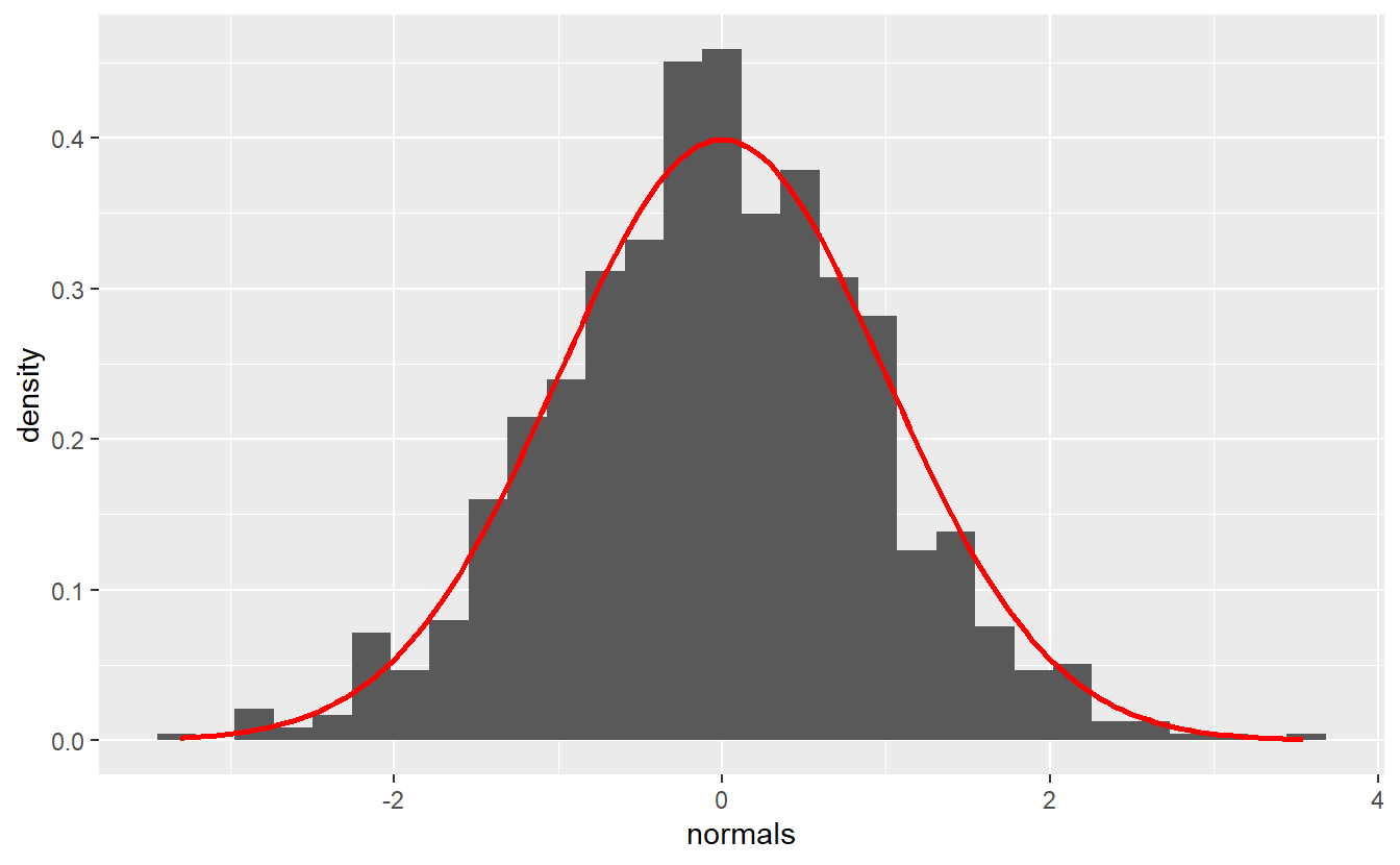
Now, let us generate a ggplot for each row in tib_normals using our new function plot_normals.
Again, we will want to use a map function instead of a for-loop to accomplish the task.
Thus, we will need a map function that can work with three arguments.
Such functions are given by pmap() and pmap_*().
Contrary to map2(), pmap() takes its input parameters via a list .l and uses the named parameters in that list as arguments for a function defined in .f.
tib_normals <- tib_normals %>%
  mutate(plots = pmap(.l = list(mu, sigma, normals), .f = plot_normals))
tib_normals
#> # A tibble: 3 x 4
#>      mu sigma normals       plots
#>   <dbl> <dbl> <list>        <list>
#> 1     1     2 <dbl [1,000]> <gg>
#> 2     2     1 <dbl [1,000]> <gg>
#> 3     3     3 <dbl [1,000]> <gg>
As you can see the plots column was computed and contains objects of type gg (as in ggplot).
Even better, this shows that we can easily save plots in a tibble which can be of advantage if for instance, we would want to generate diagnostic plots for linear models.
Plots can be easily printed by calling the tibble’s column.
To save space, I will only call the first entry of the plots column.
tib_normals$plots[[1]]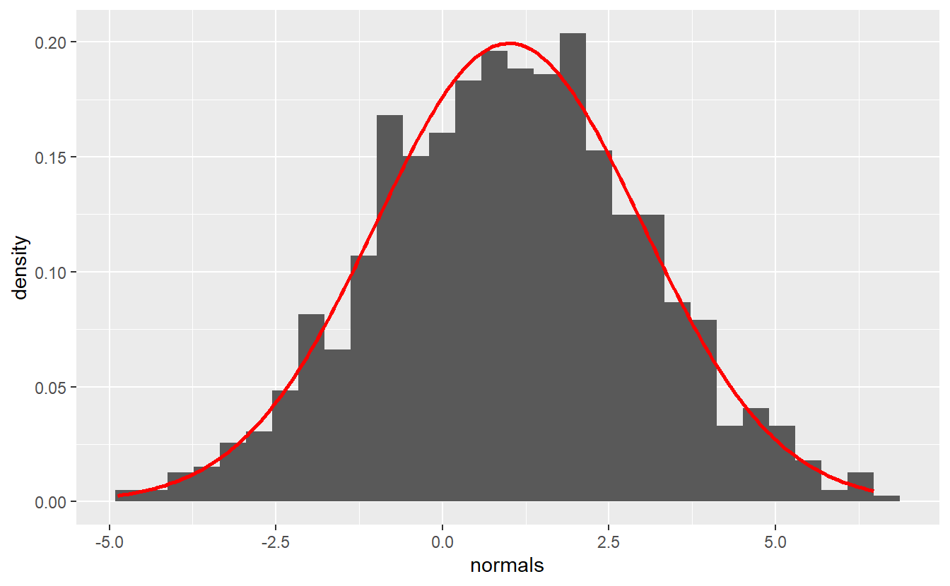
Finally, if the list passed to .l does not contain names, then one can also use an anonymous function with arguments ..1, ..2, ..3 and so on.
8.3 Exercises
8.3.1 Time measurements
Consider the following function that returns the realization from a stochastic process \(S\) on a time grid \(t = 1, 1+dt,..., T\) as a tibble consisting of the columns t and S.
simulate_process <- function(TMax = 10, dt = 0.5) {
  tibble(
    t = seq(1, TMax, dt),
    S = runif(length(t))
  ) %>%
    return()
}
simulate_process()
#> # A tibble: 19 x 2
#>       t     S
#>   <dbl> <dbl>
#> 1   1   0.220
#> 2   1.5 0.373
#> 3   2   1.00
#> 4   2.5 0.418
#> 5   3   0.268
#> 6   3.5 0.178
#> # ... with 13 more rows
Now, imagine that you want to use this function to collect 100 of the resulting tibbles by rowbinding.
Use microbenchmark::microbenchmark() to compare how long it takes to collect all of these tibbles
- via using
bind_rowsiteratively in a for-loop. - via saving the tibbles in a list and using
bind_rows()on the list. - via
map_dfr().
8.3.2 Saving and Writing Multiple Files
Often data is stored in multiple files.
With the help of map() functions we can easily read and write multiple files in a single line of code.
Use a map function,
simulate_process()andwrite_csv()to first generate 30 data filesdat1.csv,dat2.csv, …,dat30.csvin your current working directory.Read all of your .csv-files and bind them together in a single tibble using only a single pipe and no for- or while-loops.
8.3.3 Multiple Linear models
Take a look at the diamonds data set again.
diamonds
#> # A tibble: 53,940 x 10
#>   carat cut       color clarity depth table price     x     y     z
#>   <dbl> <ord>     <ord> <ord>   <dbl> <dbl> <int> <dbl> <dbl> <dbl>
#> 1  0.23 Ideal     E     SI2      61.5    55   326  3.95  3.98  2.43
#> 2  0.21 Premium   E     SI1      59.8    61   326  3.89  3.84  2.31
#> 3  0.23 Good      E     VS1      56.9    65   327  4.05  4.07  2.31
#> 4  0.29 Premium   I     VS2      62.4    58   334  4.2   4.23  2.63
#> 5  0.31 Good      J     SI2      63.3    58   335  4.34  4.35  2.75
#> 6  0.24 Very Good J     VVS2     62.8    57   336  3.94  3.96  2.48
#> # ... with 53,934 more rows
Take this data set and for each category of cut using only a single pipe and no for- or while-loops fit a linear model that explains log(price) via log(carat) and generate the diagnostic plots from autoplot().
In a separate pipe, extract the \(R^2\) statistic for each fitted model.
broom::glance() may be a helpful function.