7 Linear Models
\(\def\1{\unicode{x1D7D9}}\)
Let us start this chapter by recalling our very first model from Section 3.3.2.
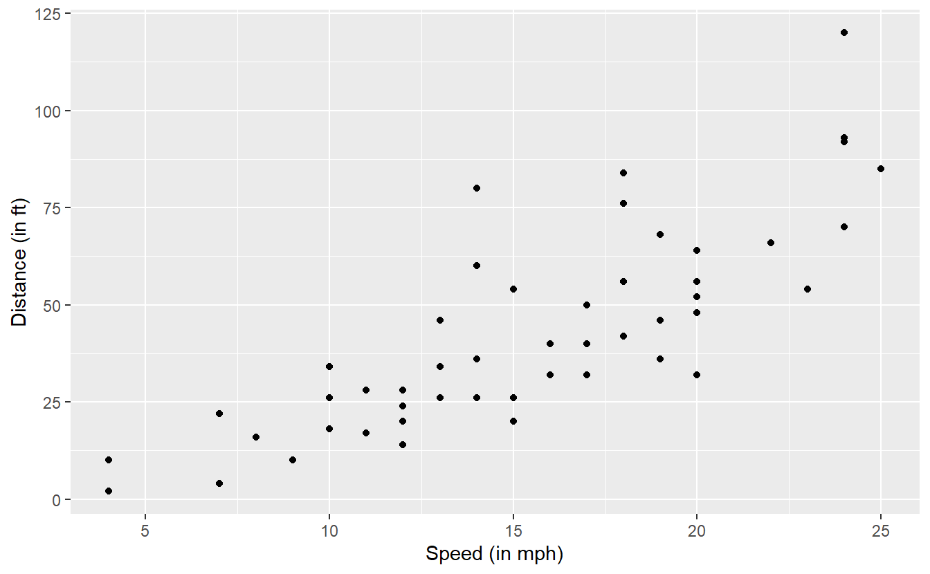
There, we looked at the cars data set which contains 50 observations of the two variables speed (speed of the car in mph) and dist (the distance it has taken the car to stop in feet).
The scatter plot of the data looks like this.
As we have already seen in Section 3.3.2, there is a physical model that describes the relationship between the distance and speed according to the red line in the following picture.
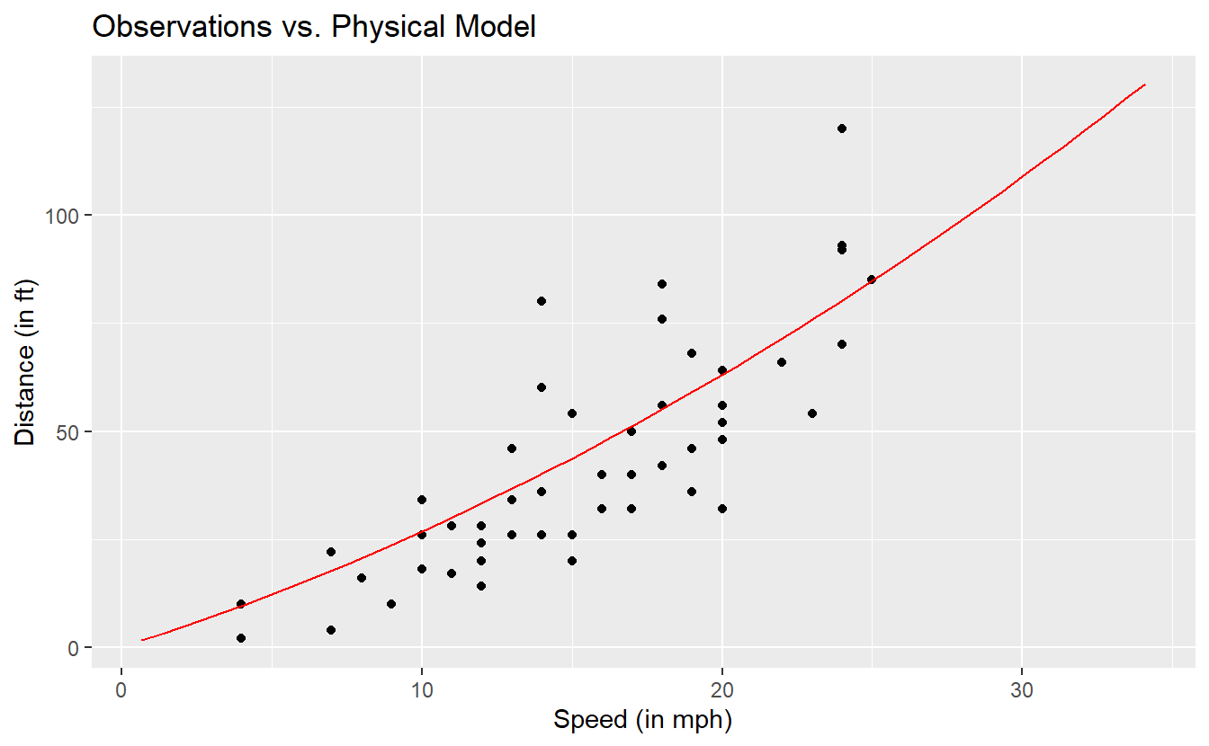
Notice that the red line does not go through all observations. Fundamentally, this is what we do, when we say that we establish a model: We try to find a function that explains the relationship between variables “sufficiently” well but leaves some room for random fluctuations.
More formally, we propose that an observation \(Y\) can be explained by another quantity \(X\) through some appropriate function \(f\). Additionally, we also allow for some random deviation \(\varepsilon\) in each observation. In total, when we try to find a model, we actually try to find a function \(f\) such that \[\begin{align*} Y = f(X) + \varepsilon. \end{align*}\] Finally, we are usually not content with any function \(f\) but require that \(f\) is chosen such that the deviations between the model prediction and the actual observations become small.
In the course of this chapter we will try to do just that. However, we will focus on so-called linear models which are characterized by considering only linear functions \(f\). On this endeavor, we will first talk about simple linear models which try to explain an observation \(Y\), also known as response, via one predictor \(X\). Afterwards, we will lift the restriction of only one predictor and talk about linear models with more than one predictor.
7.1 Simple linear model
Let us take the above data set and fit a straight line through the observations.
In ggplot2 we already learned to do this quite easily:
cars %>%
  ggplot(aes(speed, dist)) +
  geom_point() +
  geom_smooth(se = F, method = "lm")
#> `geom_smooth()` using formula 'y ~ x'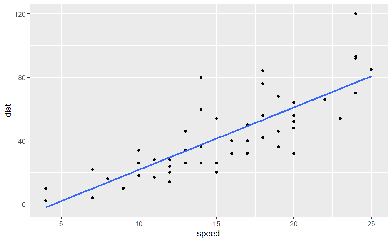
Now, the blue line represents a simple linear model since we have exactly one response variable dist and one predictor speed.
If we denote the response variable by \(Y\) and predictor variable by \(X\), we can write the model more generally as
\[\begin{align*}
Y_i = \beta_0 + \beta_1 X_i + \varepsilon_i
\end{align*}\]
for each observation \(i = 1, \ldots, n\) where \(\beta_0\), \(\beta_1 \in \mathbb{R}\) are some coefficients and \(\varepsilon_i\) are random fluctuations which we will assume to be iid. random normal variables with mean \(0\) and fixed variance \(\sigma^2\).
Also, note that for specific values from a data set we usually write small letters \(x\) resp. \(y\) and interpret these as realizations of the quantities \(X\) resp. \(Y\)62.
Now, the goal becomes to find suitable values for the intercept \(\beta_0\) and slope \(\beta_1\). Usually, these coefficients are chosen such that they minimize the residual sum of squares \[\begin{align*} \text{RSS} = \sum_{i = 1}^{n} \big(y_i - (\beta_0 + \beta_1x_i) \big)^2 \end{align*}\] which is the sum of the squared residuals, i.e. the differences between the \(i\)-th observed response variable and the \(i\)-th prediction from the linear model. This is also known as the method of least squares which is visualized in Figure 7.1 and can be explored interactively here.
. The vertical lines visualize the error of the regression slope to the real observations.](Images/least-squares-screenshot.png)
Figure 7.1: Screenshot from PhEt Interactive Simulations. The vertical lines visualize the error of the regression slope to the real observations.
With some algebra it is possible to show that the minimizers \(\hat{\beta}_0\) and \(\hat{\beta}_1\) of the RSS, i.e. the best estimates for the linear approximation, are given by \[\begin{align*} \hat{\beta}_0 &= \overline{y}_n - \hat{\beta}_1 \overline{x}_n\\[2mm] %% \hat{\beta}_1 &= \frac{ \sum_{i = 1}^{n}(x_i - \overline{x}_n)(y_i - \overline{y}_n) }{ \sum_{i = 1}^{n}(x_i - \overline{x}_n)^2 } \end{align*}\] where \(\overline{X}_n\) resp. \(\overline{y}_n\) denote the sample means of the predictors \(X\) resp. the response \(Y\).
In R, these coefficients are easily calculated with the lm() function.
Similar to specify() from the infer package it uses a formula response ~ predictorto specify what relationship we want to investigate.
lm(data = cars, dist ~ speed)
#>
#> Call:
#> lm(formula = dist ~ speed, data = cars)
#>
#> Coefficients:
#> (Intercept)        speed
#>     -17.579        3.932
Thus, we would get an intercept of \(\hat{\beta}_0 = -17.579\) and a slope of \(\hat{\beta}_1 = 3.932\). Now, this could be used to predict - according to this model - stopping distances for speeds that have not been observed in the data set. To do so, we could either compute the prediction by hand
# Extract coefficients from lm() through coefficients()
beta <- lm(data = cars, dist ~ speed) %>%
  coefficients() %>%
  unname() # Get rid of names
speed <- 4
beta[1] + beta[2] * speed
#> [1] -1.84946
or use lm()’s output in conjunction with predict().
linmod <- lm(data = cars, dist ~ speed)
# predict() requires a tibble
tib <- tibble(speed = 0:4)
predict(linmod, newdata = tib) %>%
  bind_cols(tib, prediction = .)
#> # A tibble: 5 x 2
#>   speed prediction
#>   <int>      <dbl>
#> 1     0     -17.6
#> 2     1     -13.6
#> 3     2      -9.71
#> 4     3      -5.78
#> 5     4      -1.85
Intuitively, notice that our current model cannot be right63 as it implies that low speeds correspond to negative stopping distances. Unfortunately, one drawback of a linear model is that it is not restricted to a certain range of values. In this example, it is primarily the effect of the intercept that causes the stopping distance to become negative for small speeds.
Even though it changes the above formula for the estimation of the corresponding slope, it is still easy to fit a linear model without intercept.
The exact formula is not that important, just note that a linear model without intercept can be easily achieved by adding +0 to the formula in lm64.
(linmod_woIntercept <- lm(data = cars, dist ~ speed + 0))
#>
#> Call:
#> lm(formula = dist ~ speed + 0, data = cars)
#>
#> Coefficients:
#> speed
#> 2.909
Let’s check how this new model looks compared to the real data.
beta_1 <- linmod_woIntercept %>%
  coefficients() %>%
  unname()

ggplot() +
  geom_point(data = cars, aes(speed, dist)) +
  geom_abline(slope = beta_1, col = "blue")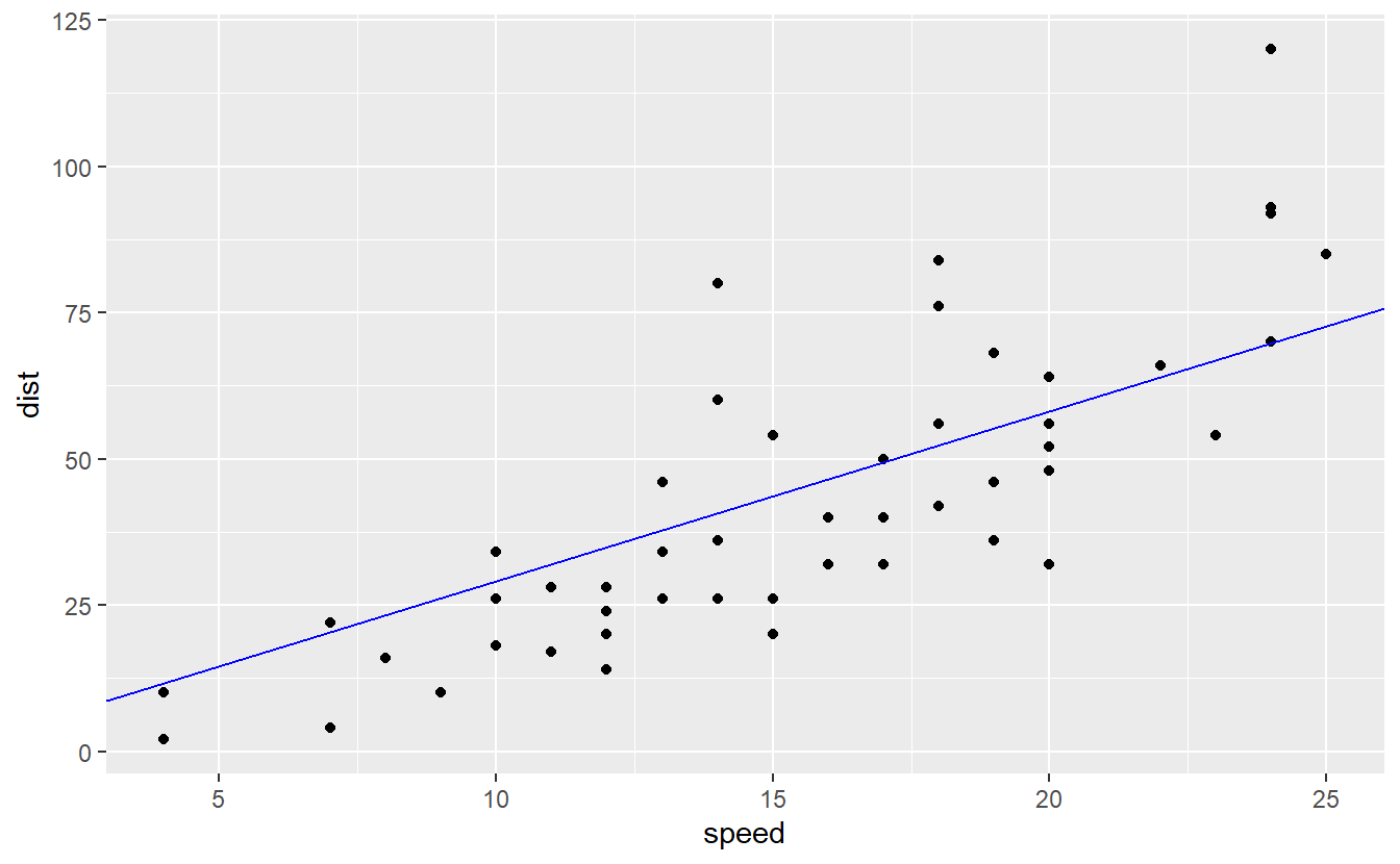
This looks also pretty decent but I suspect that the error of this second model is larger than in our original model.
For comparison’s sake, we can compute the mean squared error (MSE) of both models, i.e. we need to compute the mean of the squared residuals.
To do so for both models, we can either compute the residuals manually or use the fact that the output of lm() computes not only the coefficients but also way more than that.
In fact, the output lm() is an object of type lm which for our purposes can be treated like a regular list.
Basically, a list is a collection of vectors of possibly varying length.
Same as tibbles, the “layers” of a list can accessed either via name (using $) or index (using [[ ]] - mind the double bracket).
(example <- list(a = 1:5, c("a", "b", "c")))
#> $a
#> [1] 1 2 3 4 5
#>
#> [[2]]
#> [1] "a" "b" "c"
example$a
#> [1] 1 2 3 4 5
example[[2]][1]
#> [1] "a"
example[['a']] # combination of both name and index notation
#> [1] 1 2 3 4 5
To figure out what we can find in a list, we can simply run names().
names(linmod)
#>  [1] "coefficients"  "residuals"     "effects"       "rank"
#>  [5] "fitted.values" "assign"        "qr"            "df.residual"
#>  [9] "xlevels"       "call"          "terms"         "model"
A lot of these names do not have to mean anything to us right now, but some intuitively do, e.g. coefficients, residuals and fitted.values.
So, let us extract the residuals from our two competing linear models and compute the MSE
calc_MSE <- function(linmod) {
  MSE <- mean(linmod$residuals^2)
  return(MSE)
}

calc_MSE(linmod)
#> [1] 227.0704
calc_MSE(linmod_woIntercept)
#> [1] 259.0755
As suspected, the MSE of the model without intercept is higher. In fact, that makes sense. Since the original model could have yielded an intercept of 0 and the same slope as our second model if the RSS were in fact smaller in that case. Nevertheless, given its better interpretability the model without intercept may still be preferable even though the MSE is larger which is not to say that one could also look for a model that is both more interpretable and has a lower MSE than the original model.
For now, let’s see what more is hidden in lm()’s output.
A neat overview of essential information can be extracted via summary().
summary(linmod)
#>
#> Call:
#> lm(formula = dist ~ speed, data = cars)
#>
#> Residuals:
#>     Min      1Q  Median      3Q     Max
#> -29.069  -9.525  -2.272   9.215  43.201
#>
#> Coefficients:
#>             Estimate Std. Error t value Pr(>|t|)
#> (Intercept) -17.5791     6.7584  -2.601   0.0123 *
#> speed         3.9324     0.4155   9.464 1.49e-12 ***
#> ---
#> Signif. codes:  0 '***' 0.001 '**' 0.01 '*' 0.05 '.' 0.1 ' ' 1
#>
#> Residual standard error: 15.38 on 48 degrees of freedom
#> Multiple R-squared:  0.6511, Adjusted R-squared:  0.6438
#> F-statistic: 89.57 on 1 and 48 DF,  p-value: 1.49e-12
This output is quite loaded with information which is why we should look at all parts one by one:
Call: This is simply the
lm()function call as a reminder what linear model we’re looking at. This can be quite useful, when comparing multiple linear models.Residuals: Here, we are given an overview of the usual summary statistics. We will look at the residuals in more detail later.
-
Coefficients: For each predictor and possibly intercept you will find an estimate of the corresponding coefficient \(\beta_i\) and related quantities such as
- the standard error \(\text{SE}(\hat{\beta}_i)\) which is simply the standard deviation of the (random) estimator \(\hat{\beta}_i\) which is dependent of the unknown parameter \(\sigma^2\).
- the value of the t-statistic \[\begin{align*} \frac{\hat{\beta}_i - 0}{\widehat{\text{SE}}(\hat{\beta}_i)} \end{align*}\] which is used to test \(H_0: \beta_i = 0\) vs. \(H_0: \beta_i \neq 0\). Here, \(\widehat{\text{SE}}(\hat{\beta}_i)\) is equal to \(\text{SE}(\hat{\beta}_i)\) where the unknown parameter \(\sigma\) is estimated via \[\begin{align*} \hat{\sigma} = \sqrt{\frac{\text{RSS}}{n - 2}} = \sqrt{\frac{1}{n - 2} \sum_{i = 1}^n (y_i - \hat{y}_i)^2} \end{align*}\]
- the corresponding p-value of the t-test
- Significance codes which are displayed if a p-value falls below a certain threshold. This allows for quickly skimming which predictors (if there are multiple) may be significant, i.e. whose coefficients are significantly different from zero.
Residual standard error: This is an estimation of the unknown parameter \(\sigma\) as above.
\(R^2\)-statistic: This is a measure for “how much variability in the data set is explained by the regression”. More precisely, \[\begin{align*} R^2 = \frac{\text{TSS} - \text{RSS}}{\text{TSS}} = 1 - \frac{\text{RSS}}{\text{TSS}} \end{align*}\] where \(\text{TSS} = \sum_{i = 1}^{n} (y_i - \overline{y}_n)^2\) describes the total sum of squares which is related to the sample’s variance via a factor of \(n - 1\). Similarly, the RSS is related to the variance of the residuals, i.e. the variation that is still “unexplained” by the linear model, by the same factor (which we could easily get into both numerator and denominator).
Consequently, \(R^2\) is a measure of how much variation is “explained” by the linear model. Also, since \(R^2\) takes values between 0 and 1, this makes it easy to compare models. In general, we aim to get \(R^2\) as close as possible to 1.
Finally, the adjusted \(R^2\)-statistic is a transformation of the original \(R^2\)-statistic which tries to counterbalance the phenomenon that \(R^2\) can be increased by adding more explanatory variables even if they do not necessarily add any value to the model.F-statistic: As part of the regression an F-test is performed testing \(H_0: \beta_1 = \ldots, \beta_p = 0\) vs \(H_1: \text{not } H_0\), where \(p\) denotes the amount of predictors (so far, we have only had \(p = 1\)). The corresponding value of the F-statistic and the p-value are displayed here.
For our original model, we can see that all hypothesis tests would get rejected at a significance level of 0.05. Though, the test w.r.t. the intercept would not get rejected at a significance level of 0.01. Also, the original model has an \(R^2\)-value of 0.6511 which means that roughly 65% of the variation is explained by this model.
For comparison we can get the same information w.r.t. our second model.
summary(linmod_woIntercept)
#>
#> Call:
#> lm(formula = dist ~ speed + 0, data = cars)
#>
#> Residuals:
#>     Min      1Q  Median      3Q     Max
#> -26.183 -12.637  -5.455   4.590  50.181
#>
#> Coefficients:
#>       Estimate Std. Error t value Pr(>|t|)
#> speed   2.9091     0.1414   20.58   <2e-16 ***
#> ---
#> Signif. codes:  0 '***' 0.001 '**' 0.01 '*' 0.05 '.' 0.1 ' ' 1
#>
#> Residual standard error: 16.26 on 49 degrees of freedom
#> Multiple R-squared:  0.8963, Adjusted R-squared:  0.8942
#> F-statistic: 423.5 on 1 and 49 DF,  p-value: < 2.2e-16
As we can see, the \(R^2\)-value is much higher for our second model. This indicates that the second model is a better fit than the first one. Given the fact that the second model also offers better interpretability, let us abandon the first model and run some diagnostics on the second one to see if there may be some issues we should be aware of.
Finally, let me briefly mention that the broom package of the tidymodels metapackage offers two functions tidy() and glance() which give us the information of summary() but in a tidy format.
Of course, this might be helpful, if we want to extract specific quantities that we have seen in summary.
broom::tidy(linmod)
#> # A tibble: 2 x 5
#>   term        estimate std.error statistic  p.value
#>   <chr>          <dbl>     <dbl>     <dbl>    <dbl>
#> 1 (Intercept)   -17.6      6.76      -2.60 1.23e- 2
#> 2 speed           3.93     0.416      9.46 1.49e-12
broom::glance(linmod)
#> # A tibble: 1 x 12
#>   r.squared adj.r.squared sigma statistic  p.value    df logLik   AIC   BIC
#>       <dbl>         <dbl> <dbl>     <dbl>    <dbl> <dbl>  <dbl> <dbl> <dbl>
#> 1     0.651         0.644  15.4      89.6 1.49e-12     1  -207.  419.  425.
#> # ... with 3 more variables: deviance <dbl>, df.residual <int>, nobs <int>
7.1.1 Diagnostics with Residuals
A key assumption of a linear model is that the data exhibits an “approximate” linear relationship between response and predictor. The idea of only an approximate linear relationship is expressed in the fact that the residuals \(\varepsilon_i\), \(i = 1, \ldots, n\), allow for some random deviation from an exact linear relationship. Nevertheless, we do not allow the residuals to be arbitrarily random because we assume that they are iid. and normally distributed with mean 0 and variance \(\sigma^2\).
Implicitly, this suggests that we can detect a highly non-linear relationship if we look at the residuals after a linear fit. Thus, it is wise to look at the distribution of the residuals after we have fitted a linear model. In this regard, a residuals vs. fitted plot is a common diagnostic tool to check for potential problems with our regression.
As the name implies, the idea is to draw a scatter plot using the residuals \(\varepsilon_i\) and the corresponding fitted values \(\hat{y}_i\). If these points look randomly scattered around 0 with constant variance across the whole range of fitted values, then we can assume that our linear model works somewhat well. In short, we have to be on the lookout for any patterns.
res <- linmod_woIntercept$residuals
fits <- linmod_woIntercept$fitted.values

ggplot(mapping = aes(fits, res)) +
  geom_point() +
geom_hline(yintercept = 0, linetype = 2) 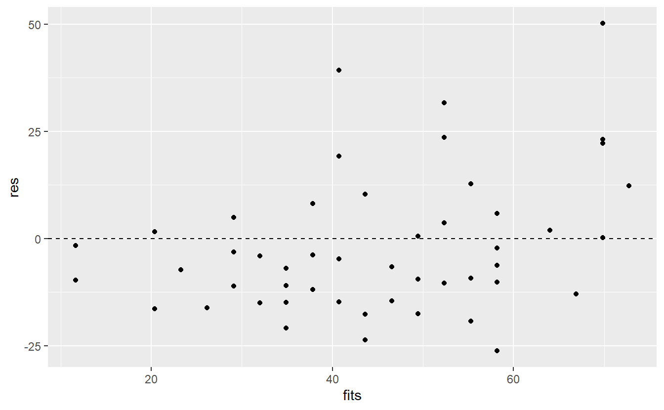
Here, it looks like there are way more points below zero which does not speak in favor of a good fit. Additionally, there may be a trend suggesting that the residuals increase as the fitted values increase. Let’s see if a smoothed line can shed some light on this.
ggplot(mapping = aes(fits, res)) +
  geom_point() +
  geom_hline(yintercept = 0, linetype = 2) +
  geom_smooth()
#> `geom_smooth()` using method = 'loess' and formula 'y ~ x'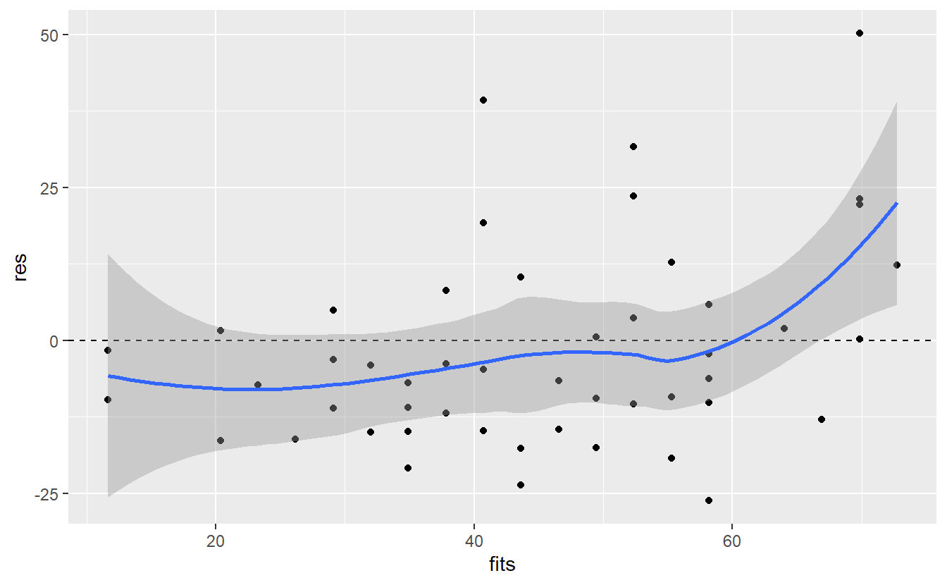
Ideally, the blue line corresponds with the dashed line which is not the case here65. Also, as we suspected there is an increase in the residuals towards the right end of the plot. All in all, this may suggest that there is still something that we are missing in our model.
A similiar plot that is quite common uses so-called standardized residuals instead of the regular residuals. These are calculated through dividing each residual \(\varepsilon_i\) by \(\hat{\sigma} \sqrt{1 - h_i}\) where \(h_i\) describes the so-called leverage of the \(i\)-th observation.
At this point, let me note that we will cover the leverage \(h_i\) of the observation in more detail very soon. For now, I merely want to point out that \(\hat{\sigma} \sqrt{1 - h_i}\) is used for normalization because \(\text{Var}(\hat{\varepsilon}_i) = \sigma (1 - h_i)\) where \(\hat{\varepsilon_i}\), which can be computed as the difference of the real observation \(y_i\) and the corresponding prediction \(\hat{y}_i\), denotes the estimator of the theoretical residual \(\varepsilon\).
Also, if we were to normalize the (estimated) residuals using only \(\hat{\sigma}\), then we would compute the studentized residuals. Finally, the square roots of the absolute value of the standardized residuals are plotted against the fitted values.
# lm.influence computes leverage
hi <- lm.influence(linmod_woIntercept, do.coef = F)$hat
# Compute standardized residuals
n <- length(hi)
sigma <- sqrt(1 / (n - 2) * sum(res^2))
standardized_res <- res / (sigma * sqrt(1 - hi))
root_standard_res <- sqrt(abs(standardized_res))

ggplot(mapping = aes(fits, root_standard_res)) +
  geom_point() +
  geom_smooth()
#> `geom_smooth()` using method = 'loess' and formula 'y ~ x'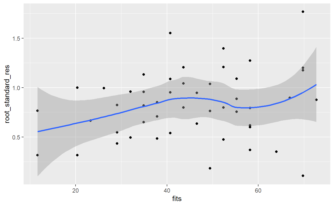
Here, the message of the plot is the same as with the regular residuals: It looks like the error is increasing as the fitted value increase. Maybe an additional predictor would help with that.
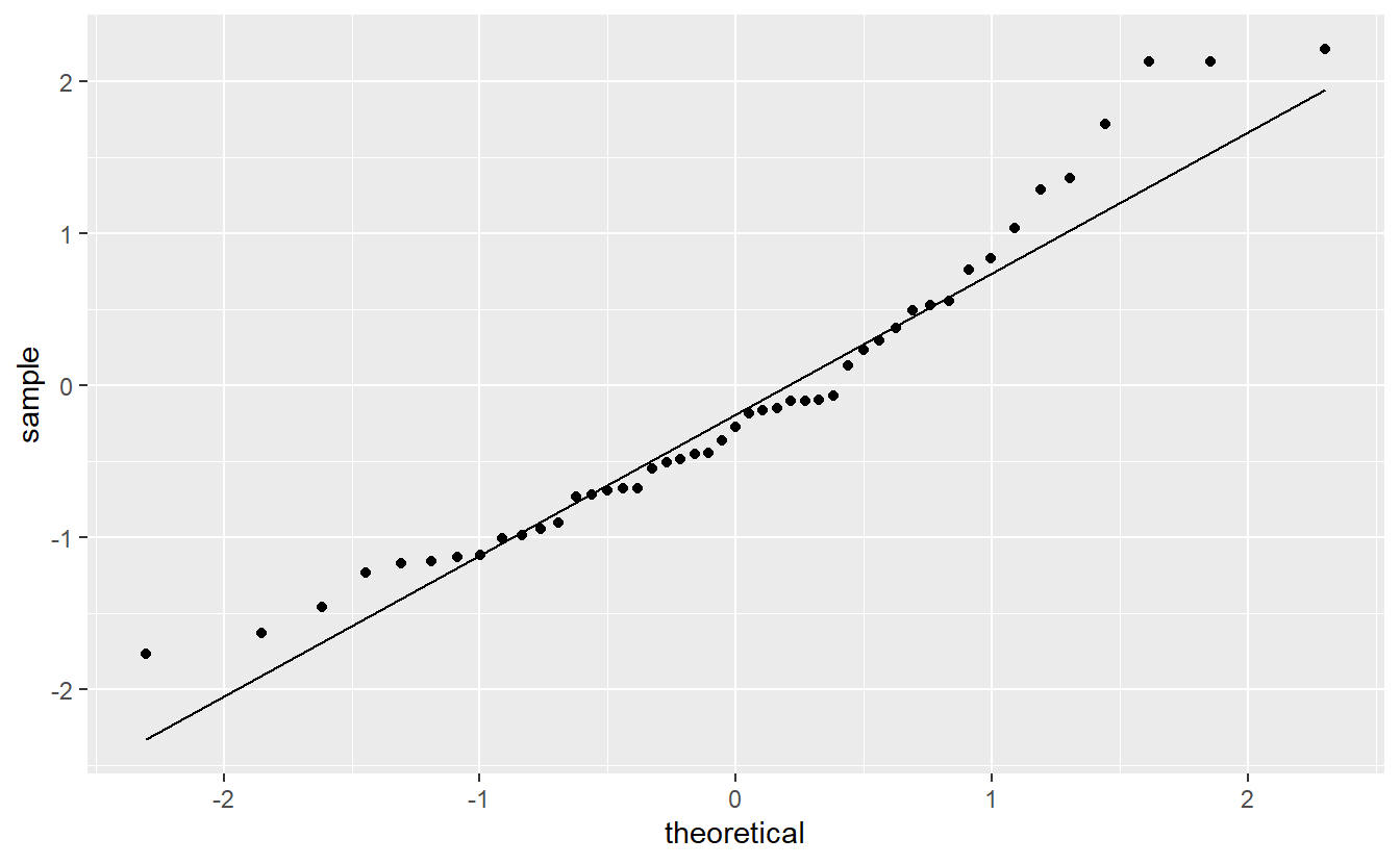
For now, let us check if the normality assumption holds. In practice, this is usually done via a qq-plot to compare the quantiles of the standard normal distribution to the quantiles of the standardized residuals.
ggplot(mapping = aes(sample = standardized_res)) +
  geom_qq() +
  geom_qq_line()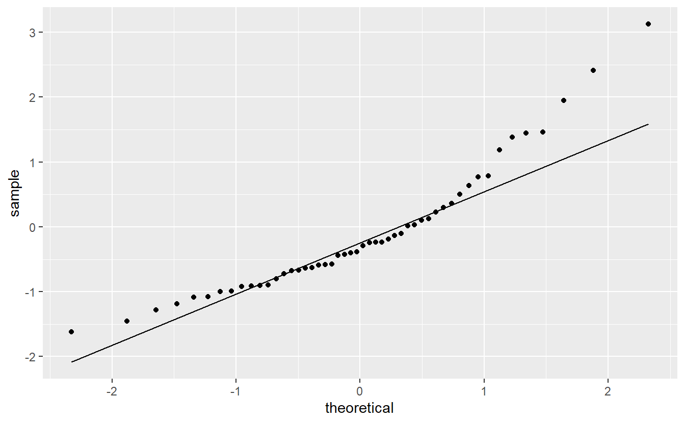
This looks somewhat ok, but not great either. Also on the right of this picture, we can see that there are a couple of points that there are larger than expected which brings us to our next point.
It appears that some of the residuals are extraordinarily large. For instance, the following three residuals (indicated in red) look larger than most of the others.
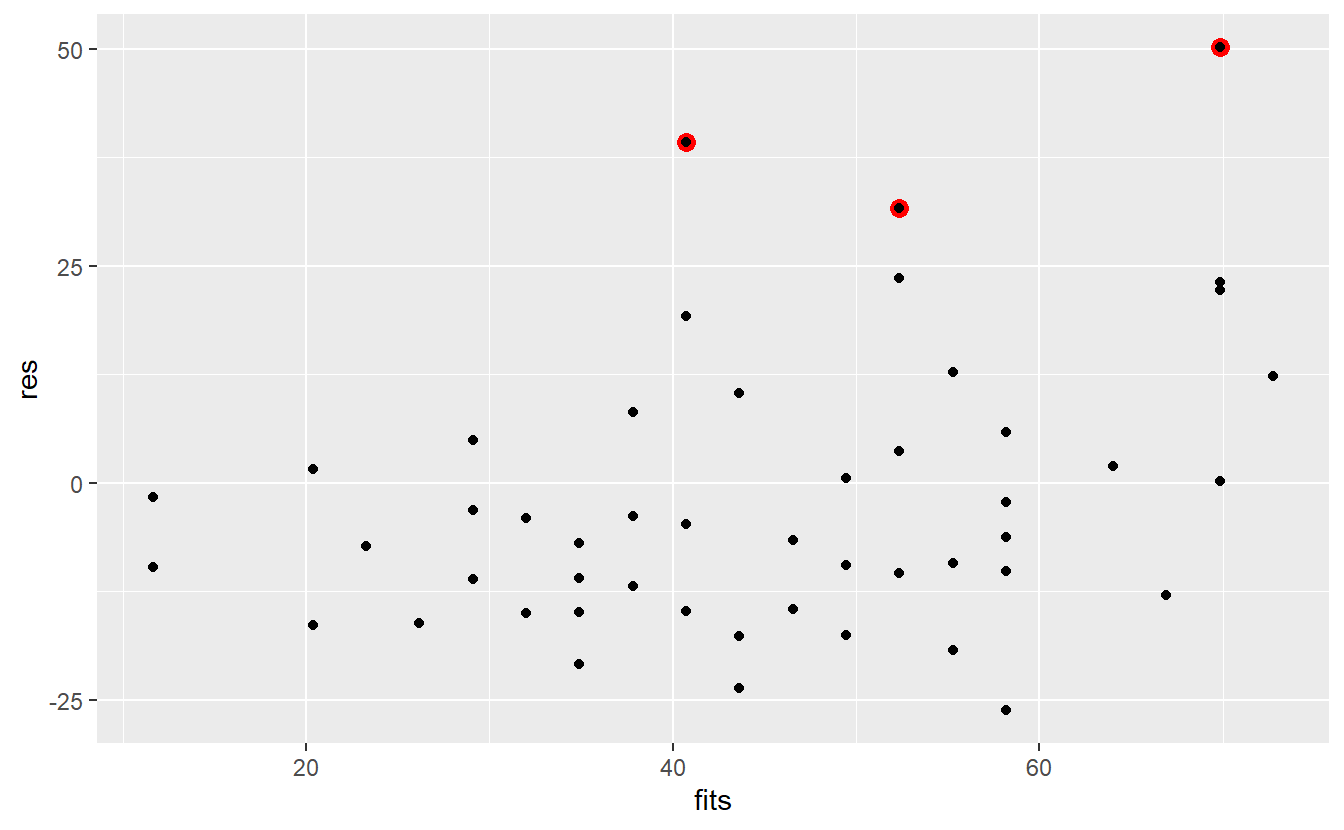
With respect to our initial data set, these residuals correspond to the following observations.
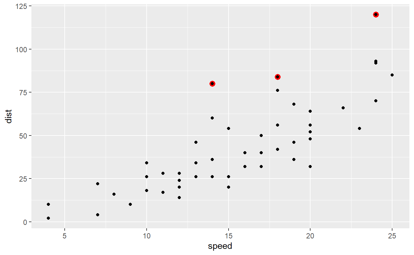 Observations like these, i.e. unusually large ones, are what we usually call outliers.
Of course, outliers do not necessarily have to be large.
Often, it is also uncharacteristically small observations which may be a reason for concern.
Observations like these, i.e. unusually large ones, are what we usually call outliers.
Of course, outliers do not necessarily have to be large.
Often, it is also uncharacteristically small observations which may be a reason for concern.
Naturally, outliers may have an impact on a linear model’s quality of fit. This is why - in a lot of situations - one tries to filter them out of the data set before one runs the regression. Often, this is motivated by simply assuming an error in the collection of the data.
Though, there are also situations where it it not appropriate to ignore outliers. For instance, in extreme value statistics it is usually the extremes we are interested in. Thus, filtering out the extreme observations may conflict with whatever it is we try to investigate. In our case, let us simply remove the previously indicated observations to get a feeling for how much they may impact our regression.
linmod_woOutliers <- cars %>%
  as_tibble() %>%
  mutate(
    fits = predict(linmod_woIntercept),
    res = dist - fits,
    rank = rank(res)
  ) %>%
  filter(rank <= 47) %>%
  lm(data = ., dist ~ speed + 0)

summary(linmod_woOutliers)
#>
#> Call:
#> lm(formula = dist ~ speed + 0, data = .)
#>
#> Residuals:
#>     Min      1Q  Median      3Q     Max
#> -22.352 -10.405  -3.482   5.495  27.777
#>
#> Coefficients:
#>       Estimate Std. Error t value Pr(>|t|)
#> speed   2.7176     0.1155   23.52   <2e-16 ***
#> ---
#> Signif. codes:  0 '***' 0.001 '**' 0.01 '*' 0.05 '.' 0.1 ' ' 1
#>
#> Residual standard error: 12.72 on 46 degrees of freedom
#> Multiple R-squared:  0.9233, Adjusted R-squared:  0.9216
#> F-statistic: 553.4 on 1 and 46 DF,  p-value: < 2.2e-16
Judging from the \(R^2\)-value, our model without these outliers is better as it increased the \(R^2\)-value from 0.8963 to 0.9233. Also, notice that the slope estimate changed from 2.9091 to 2.7176 which is not a measure of the model’s accuracy but nevertheless shows how only three observations can influence the estimation. Further, the new model’s qq-plot also looks a bit better.
Now that we have understood that outliers can be an influence on a regression’s quality, we should think of a more neutral way to determine what deviations constitute an outlier and which do not. This is where the standardized residuals come into play again. As a rule of thumb one often considers observations whose standardized residual are below -3 or above 3 to be outliers. In our case this means that the following point is an outlier.
# lm.influence computes leverage
hi <- lm.influence(linmod_woIntercept, do.coef = F)$hat
res_woIntercept <- linmod_woIntercept$residuals
# Compute standardized residuals
n <- length(hi)
sigma <- sqrt(1 / (n - 2) * sum(res_woIntercept^2))
standardized_res <- res_woIntercept / (sigma * sqrt(1 - hi))

cars %>%
  as_tibble() %>%
  mutate(
    standardized_res = standardized_res,
    outlier = ifelse(abs(standardized_res) > 3, T, F)
  ) %>%
  ggplot() +
  geom_point(aes(speed, dist, col = outlier), show.legend = F) +
  scale_color_manual(values = c("black", "red"))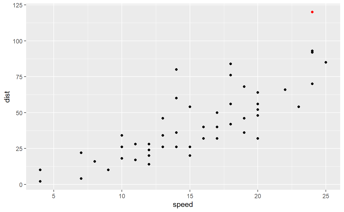
If we remove this outlier, this gives us the following linear model.
linmod_woOutliers <- cars %>%
  as_tibble() %>%
  mutate(standardized_res = standardized_res) %>%
  filter(abs(standardized_res) <= 3) %>%
  lm(data = ., dist ~ speed + 0)

summary(linmod_woOutliers)
#>
#> Call:
#> lm(formula = dist ~ speed + 0, data = .)
#>
#> Residuals:
#>     Min      1Q  Median      3Q     Max
#> -24.279 -10.721  -4.279   5.349  40.605
#>
#> Coefficients:
#>       Estimate Std. Error t value Pr(>|t|)
#> speed   2.8139     0.1304   21.59   <2e-16 ***
#> ---
#> Signif. codes:  0 '***' 0.001 '**' 0.01 '*' 0.05 '.' 0.1 ' ' 1
#>
#> Residual standard error: 14.66 on 48 degrees of freedom
#> Multiple R-squared:  0.9066, Adjusted R-squared:  0.9047
#> F-statistic: 465.9 on 1 and 48 DF,  p-value: < 2.2e-16
Again, removing this outlier improved the \(R^2\)-value and changed the slope estimation w.r.t. to our original model. Now, notice that outliers are observations whose response variable \(y\) deviates a lot from a linear model’s predicted response variable \(\hat{y}\). Similarly, in a given data set there can be observations whose predictor \(x\) is quite different from the other observations.
For instance, in our example we observe speeds that are ranged within
range(cars$speed)
#> [1]  4 25
So, if we were to add an observation with speed 50, then this observation would be quite different from the other observations and might have a tremendous influence on the estimated parameters (depending on the corresponding dist value).
Also, a point like this would then have a large leverage on the regression and be called leverage point.
In simple linear regression the leverage of the \(i\)-th observation can be computed by \[\begin{align*} h_i = \frac{1}{n} + \frac{ (x_i - \overline{x}_n)^2 }{\sum_{j = 1}^{n} (x_j - \overline{x}_n)^2}. \end{align*}\] In a way, this formula tries to measure how much each observation deviates from the average observation.
Further, the average leverage for all observations is equal to \((p + 1)/ n\) where \(p\) is the amount of predictors we use (so far \(p\) was always equal to 1). Thus, a point may be a leverage point if its leverage is much larger than \((p + 1) / n\). Some rules of thumb suggest to use \(2(p + 1)/n\) or \(3(p+1)/n\) as threshold to judge whether an observation constitutes a leverage point.
As before, leverages are often observed through a diagnostic plot. In this case, it is common to plot the standardized residuals against the leverage. This enables us to detect potential observations that are both outliers and have high leverage which is usually a bad combination.
#> `geom_smooth()` using method = 'loess' and formula 'y ~ x'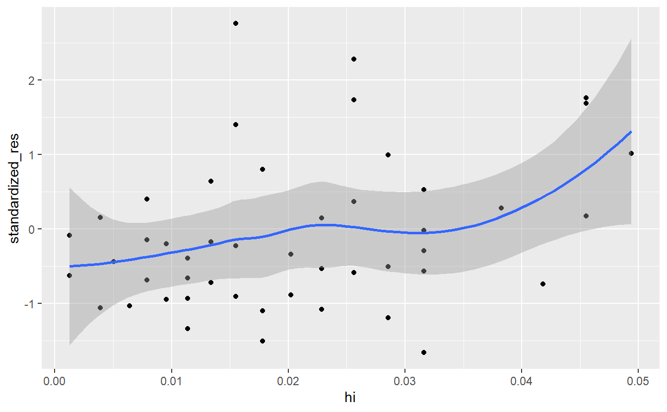
In this case \(2(p + 1)/n\) equals to 0.0816327 so we do not need to remove any points.
Finally, all of these common plots can be created automatically from an lm object.
Loading the ggfortify package lets the command autoplot() know how to interpret an lm object and generate all four diagnostic plots in a single line of code.
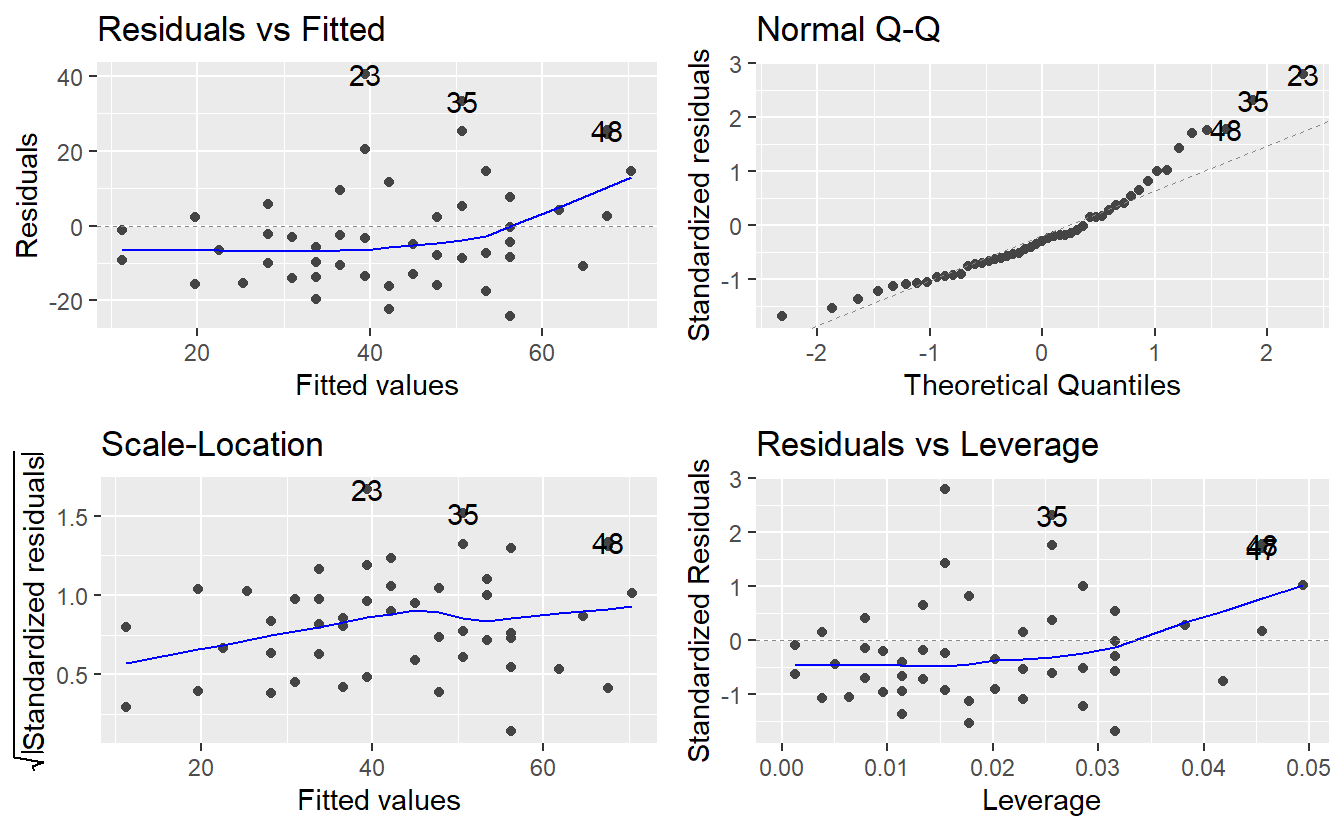
As you can see, autoplot() also highlights some observations by their row numbers.
This can be helpful to investigate some of these observations in more detail.
However, we will deal with the more pressing issue of increasing residuals now.
7.2 Linear models
To make the transition from a single to multiple predictors, it is convenient to rewrite our simple linear regression equations \[\begin{align*} Y_i = \beta_0 + \beta_1 x_i + \varepsilon_i, \quad i = 1, \ldots, n \end{align*}\] into one single equation using matrix notation. This yields the equation \[\begin{align*} Y = X\beta + \varepsilon, \end{align*}\] where \[\begin{align*} Y = \begin{pmatrix} Y_1 \\ \vdots \\ Y_n \end{pmatrix}, \quad % X = \begin{pmatrix} 1 & X_1 \\ \vdots & \vdots\\ 1 & X_n \end{pmatrix}, \quad % \beta = \begin{pmatrix} \beta_0 \\ \beta_1 \end{pmatrix} \quad \text{ and } \quad \varepsilon = \begin{pmatrix} \varepsilon_1 \\ \vdots \\ \varepsilon_n \end{pmatrix}. \end{align*}\]
Through some algebraic shuffling around, it can be shown that the least squares estimator of \(\beta\) can be written as \[\begin{align*} \hat{\beta} = \begin{pmatrix} \hat{\beta}_0 \\ \hat{\beta}_1 \end{pmatrix} = (X^\top X)^{-1}X^{\top}Y \end{align*}\] where \(X^\top\) denotes the transpose of matrix \(X\) which is often called design matrix.
Thankfully, this formula generalizes well such that the least squares estimator of \(\beta\) for models of the form \[\begin{align*} Y_i = \beta_0 + \beta_1 X_i^{(1)} + \ldots + \beta_p X_i^{(p)} + \varepsilon_i, \quad i = 1, \ldots, n, \end{align*}\] i.e. linear models with \(p \in \mathbb{N}\) predictors, can be computed using the same formula \[\begin{align*} \hat{\beta} = \begin{pmatrix} \hat{\beta}_0 \\ \vdots \\ \hat{\beta}_p \end{pmatrix} = (X^\top X)^{-1}X^{\top}Y \quad \text{ with } X = \begin{pmatrix} 1 & X_1^{(1)} & \cdots & X_1^{(p)} \\ \vdots & \vdots & \ddots & \vdots \\ 1 & X_n^{(1)} & \cdots & X_n^{(p)} \end{pmatrix} \end{align*}\]
Luckily, because most of the concepts that we have covered for simple linear regression are practically the same for multiple linear regression, we can dive right into using more than one predictor for our previous data set. Since it looked like the errors were increasing as the fitted values were increasing, a common remedy for behavior like that is to incorporate a quadratic term into our model.
A quadratic term you say? I thought we are doing only linear models here. That’s right. The term linear model refers to the fact that our parameters \(\beta_i\) play only a linear role, i.e. we could not use a model like \(Y_i = \beta_0 + \beta^2_1 x_i + \varepsilon_i\) and call it linear. However, the predictors may be whatever they want to be.
If you have trouble grasping this you may think about creating another variable in a data set by simply squaring an already existing variable. For instance, in our case this may look like
cars %>%
  as_tibble() %>%
  mutate(new_speed = speed^2)
#> # A tibble: 50 x 3
#>   speed  dist new_speed
#>   <dbl> <dbl>     <dbl>
#> 1     4     2        16
#> 2     4    10        16
#> 3     7     4        49
#> 4     7    22        49
#> 5     8    16        64
#> 6     9    10        81
#> # ... with 44 more rows
Now, maybe, it feels less awkward to incorporate this new variable as part of a simple linear model instead of using the original variable speed.
After all, it is now only another variable in a data set.
Who cares whether it is the square of something else?66
In R, it is straight-forward to fit a model using more than one predictor.
All we have to do is67 extend the formula in lm().
linMod_quad <- lm(data = cars, dist ~ speed + speed^2 + 0)
summary(linMod_quad)
#>
#> Call:
#> lm(formula = dist ~ speed + speed^2 + 0, data = cars)
#>
#> Residuals:
#>     Min      1Q  Median      3Q     Max
#> -26.183 -12.637  -5.455   4.590  50.181
#>
#> Coefficients:
#>       Estimate Std. Error t value Pr(>|t|)
#> speed   2.9091     0.1414   20.58   <2e-16 ***
#> ---
#> Signif. codes:  0 '***' 0.001 '**' 0.01 '*' 0.05 '.' 0.1 ' ' 1
#>
#> Residual standard error: 16.26 on 49 degrees of freedom
#> Multiple R-squared:  0.8963, Adjusted R-squared:  0.8942
#> F-statistic: 423.5 on 1 and 49 DF,  p-value: < 2.2e-16
Unfortunately, this did not do what we wanted it to do.
Nothing changed.
This happened because the syntax ^2 in a formula is reserved for something else.
If we want to use a squared variable, then we have to surround it by I().
linMod_quad <- lm(data = cars, dist ~ speed + I(speed^2) + 0)
summary(linMod_quad)
#>
#> Call:
#> lm(formula = dist ~ speed + I(speed^2) + 0, data = cars)
#>
#> Residuals:
#>     Min      1Q  Median      3Q     Max
#> -28.836  -9.071  -3.152   4.570  44.986
#>
#> Coefficients:
#>            Estimate Std. Error t value Pr(>|t|)
#> speed       1.23903    0.55997   2.213  0.03171 *
#> I(speed^2)  0.09014    0.02939   3.067  0.00355 **
#> ---
#> Signif. codes:  0 '***' 0.001 '**' 0.01 '*' 0.05 '.' 0.1 ' ' 1
#>
#> Residual standard error: 15.02 on 48 degrees of freedom
#> Multiple R-squared:  0.9133, Adjusted R-squared:  0.9097
#> F-statistic: 252.8 on 2 and 48 DF,  p-value: < 2.2e-16
Judging from the \(R^2\)-value this new model seems to be the best fit so far. Let’s also check the diagnostic plots.
autoplot(linMod_quad)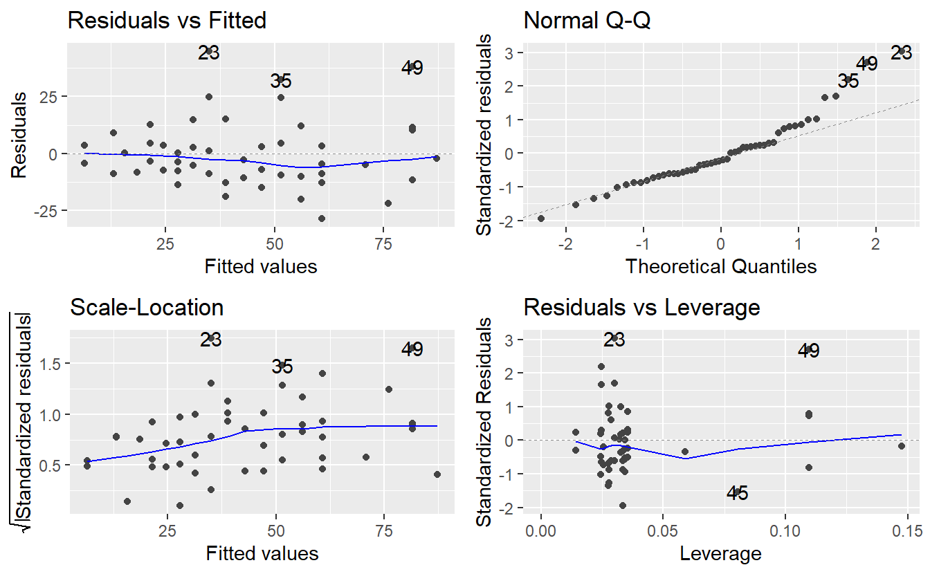
The residuals look better now. At least, there is way less trend detectable in the residuals, so adding the quadratic term indeed helped. Notice that we used the whole data set for the fit here. Consequently, checking for outliers and leverage points may improve the results even further. Now, let us look at a different data set and see what more trouble we can run in with linear regressions.
7.2.1 Categorical Predictors
The following example is inspired by Chapter 24.2 in R for Data Science by Hadley Wickham. The full analysis which this part is based on can be found in that book.
Our favorite plotting package ggplot2 comes with a data set called diamonds which “contain the prices and other attributes of almost 54,000 diamonds”.
Let us take a sneak peak at the data
diamonds
#> # A tibble: 53,940 x 10
#>   carat cut       color clarity depth table price     x     y     z
#>   <dbl> <ord>     <ord> <ord>   <dbl> <dbl> <int> <dbl> <dbl> <dbl>
#> 1  0.23 Ideal     E     SI2      61.5    55   326  3.95  3.98  2.43
#> 2  0.21 Premium   E     SI1      59.8    61   326  3.89  3.84  2.31
#> 3  0.23 Good      E     VS1      56.9    65   327  4.05  4.07  2.31
#> 4  0.29 Premium   I     VS2      62.4    58   334  4.2   4.23  2.63
#> 5  0.31 Good      J     SI2      63.3    58   335  4.34  4.35  2.75
#> 6  0.24 Very Good J     VVS2     62.8    57   336  3.94  3.96  2.48
#> # ... with 53,934 more rows
For convenience, we will focus on the variables price, carat (weight) and cut (quality) here.
(tib_diam <- diamonds %>% select(price, carat, cut))
#> # A tibble: 53,940 x 3
#>   price carat cut
#>   <int> <dbl> <ord>
#> 1   326  0.23 Ideal
#> 2   326  0.21 Premium
#> 3   327  0.23 Good
#> 4   334  0.29 Premium
#> 5   335  0.31 Good
#> 6   336  0.24 Very Good
#> # ... with 53,934 more rows
Also, let’s check whether there are any missing values.
tib_diam %>%
  mutate(across(.fns = is.na)) %>%
  summarise(across(.fns = sum))
#> # A tibble: 1 x 3
#>   price carat   cut
#>   <int> <int> <int>
#> 1     0     0     0
It appears that we are in luck and we do not have to deal with missing values.
Now, let’s look at the levels of cut.
tib_diam %>%  pull(cut) %>% unique()
#> [1] Ideal     Premium   Good      Very Good Fair
#> Levels: Fair < Good < Very Good < Premium < Ideal
As you can see, the variable cut has 5 levels which can be ordered as depicted.
The fact that this ordering is displayed shows that the cut column in tib_diam is not only a factor vector but an ordered factor.
tib_diam %>% pull(cut) %>% is.ordered()
#> [1] TRUE
This becomes important when we try to run a linear regression of the price based on carats and the quality of the cut.
lm(data = tib_diam, price ~ carat + cut)
#>
#> Call:
#> lm(formula = price ~ carat + cut, data = tib_diam)
#>
#> Coefficients:
#> (Intercept)        carat        cut.L        cut.Q        cut.C        cut^4
#>    -2701.38      7871.08      1239.80      -528.60       367.91        74.59
This output is somewhat weird and hard to interpret.
Here, lm() tries to use the fact that cut is ordered and tries to convert it into something resembling numerical predictors relating to “linear”, “quadratic”, “cubic” end “fourth power influence of cut on the response”.
This is hard to interpret, so we will need to artificially get rid of the ordering.
linmod_diam <- tib_diam %>%
  mutate(cut = factor(cut, ordered = F)) %>%
  lm(data = ., price ~ carat + cut)
summary(linmod_diam)
#>
#> Call:
#> lm(formula = price ~ carat + cut, data = .)
#>
#> Residuals:
#>      Min       1Q   Median       3Q      Max
#> -17540.7   -791.6    -37.6    522.1  12721.4
#>
#> Coefficients:
#>              Estimate Std. Error t value Pr(>|t|)
#> (Intercept)  -3875.47      40.41  -95.91   <2e-16 ***
#> carat         7871.08      13.98  563.04   <2e-16 ***
#> cutGood       1120.33      43.50   25.75   <2e-16 ***
#> cutVery Good  1510.14      40.24   37.53   <2e-16 ***
#> cutPremium    1439.08      39.87   36.10   <2e-16 ***
#> cutIdeal      1800.92      39.34   45.77   <2e-16 ***
#> ---
#> Signif. codes:  0 '***' 0.001 '**' 0.01 '*' 0.05 '.' 0.1 ' ' 1
#>
#> Residual standard error: 1511 on 53934 degrees of freedom
#> Multiple R-squared:  0.8565, Adjusted R-squared:  0.8565
#> F-statistic: 6.437e+04 on 5 and 53934 DF,  p-value: < 2.2e-16
Now, the coefficients are a bit easier to interpret. In this case, the coefficients may translate into something like \[\begin{align*} \text{price}_i &= -3875 + 7871 \cdot \text{carat}_i \\ &+ 1120 \cdot \1\{\text{cut}_i = \text{ Good} \} \\ &+ 1510 \cdot \1\{\text{cut}_i = \text{ Very Good} \} \\ &+ 1439 \cdot \1\{\text{cut}_i = \text{ Premium} \} \\ &+ 1801 \cdot \1\{\text{cut}_i = \text{ Ideal} \} + \varepsilon_i \end{align*}\] Thus, one can interpret this as that the price of a diamond increases by a fixed amount depending on what quality the diamond falls in. For instance, in this model the price of a diamond that is only “fair” will get no additional amount added to its price. On the other hand, if the quality of the same diamond is “good”, then the price will increase by 1120 and so on.
In effect, lm() has created dummy variables to encode the categorical variables.
Of course, there are other ways to encode categorical variables but here we will stick to the default option.
Now, if we look closely at the results and recall that the “premium” diamonds are supposed to be superior to “very good” diamonds, it is hard not to wonder why the price increases more for diamonds of the latter kind than it does for diamonds of the former kind. Therefore, we should look at our diagnostic plots and see if we can detect where things go awry.
autoplot(linmod_diam)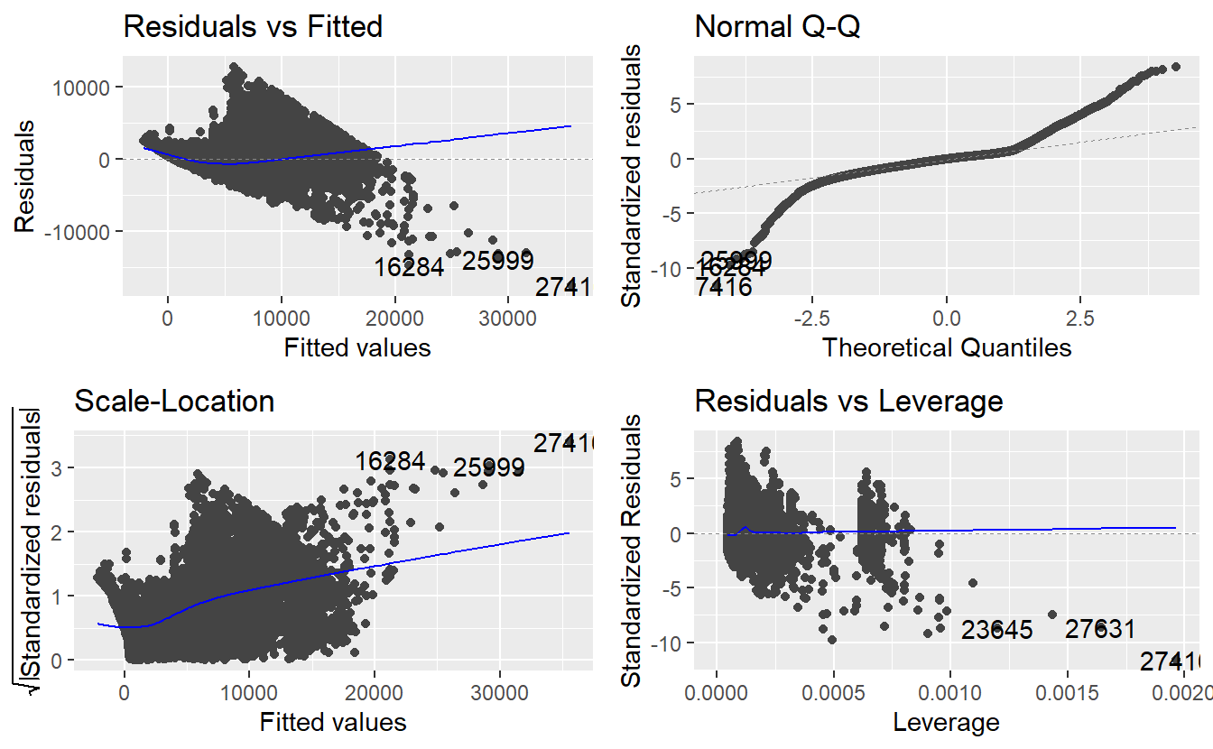
Obviously, we have a severe problem with overplotting here because we have a large amount of data points. Of course, we can still detect that there is some kind of pattern in the residuals, so let us try to depict this in a more sophisticated manner.
tib_diam <- tib_diam %>%
mutate(
res = linmod_diam$residuals,
fits = linmod_diam$fitted.values
)
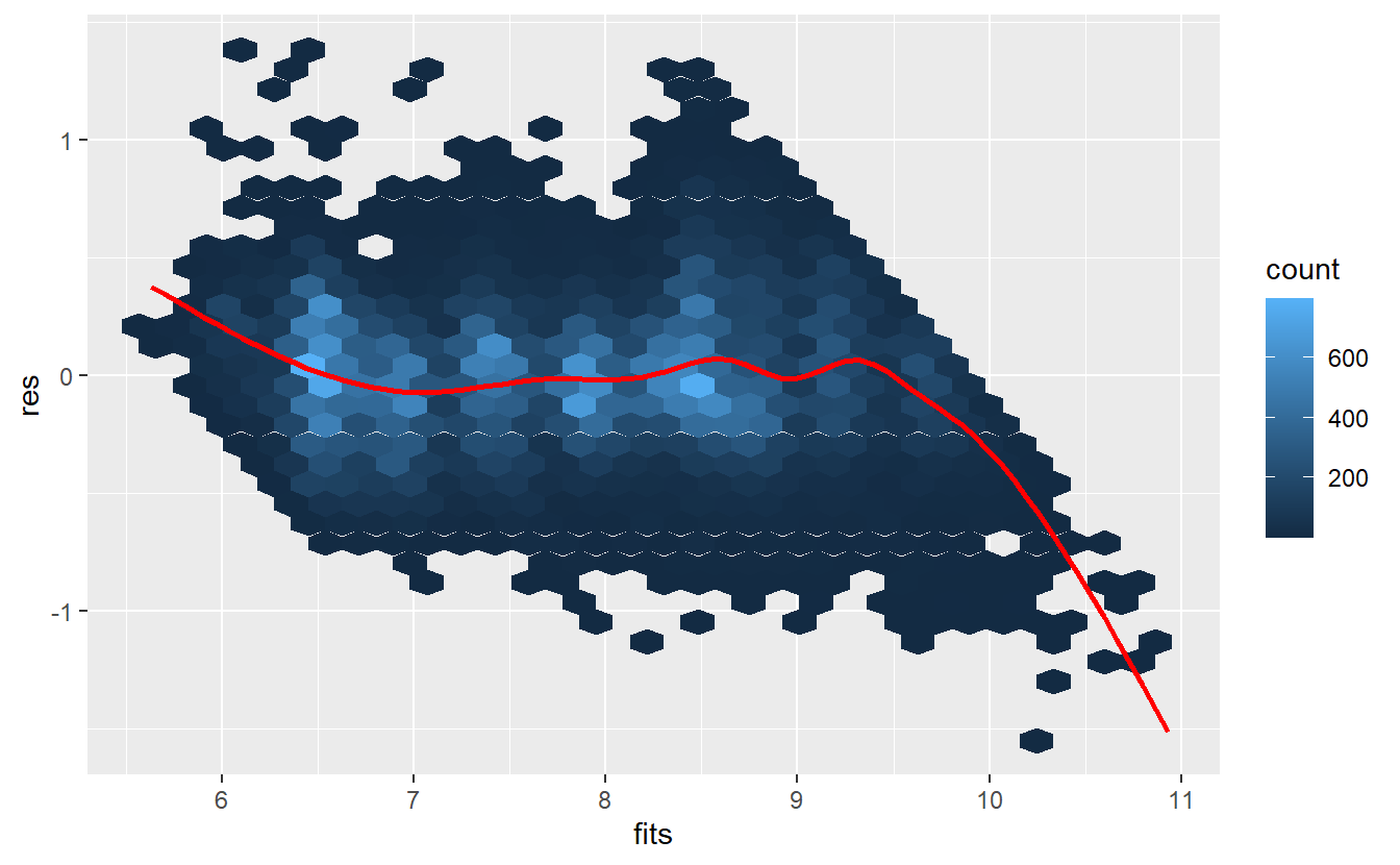
tib_diam %>%
ggplot(aes(fits, res)) +
geom_hex()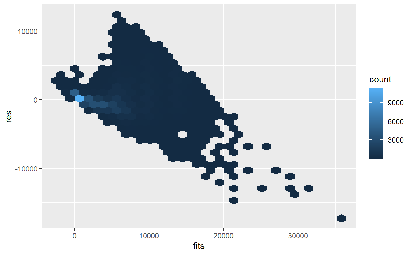
As said before, clearly this is not randomly scattered. Maybe we should have taken a look at the observations before we started to fit a linear model to it.
tib_diam %>%
  ggplot(aes(carat, price)) +
  geom_hex() +
  geom_smooth(col = "red", se = F) +
  facet_wrap(vars(cut), scale = "free")
#> `geom_smooth()` using method = 'gam' and formula 'y ~ s(x, bs = "cs")'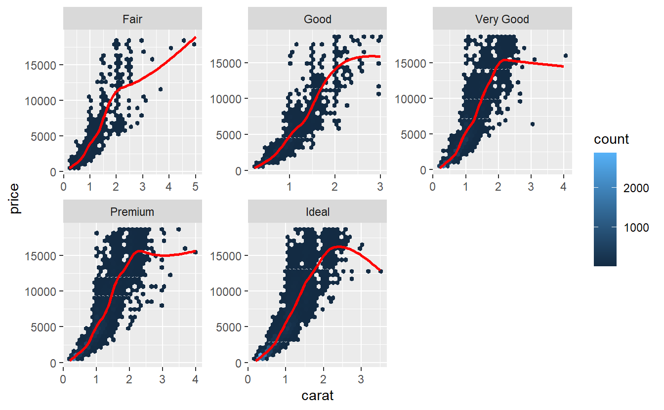
Especially, the very good and upwards diamonds look more parabolic than they do look linear. Often, one tries to remedy the non-linearity by transforming the variables before applying a linear regression to it. Prices can often be log-transformed to achieve linearity.
Quite frequently, this is due to the fact that a data set may contain both very low and very high prices and the logarithm makes the differences less extreme. Let’s see what happens here.
tib_diam %>%
  ggplot(aes(carat, price)) +
  geom_hex() +
  geom_smooth(col = "red", se = F) +
  facet_wrap(vars(cut), scale = "free") +
  scale_y_log10()
#> `geom_smooth()` using method = 'gam' and formula 'y ~ s(x, bs = "cs")'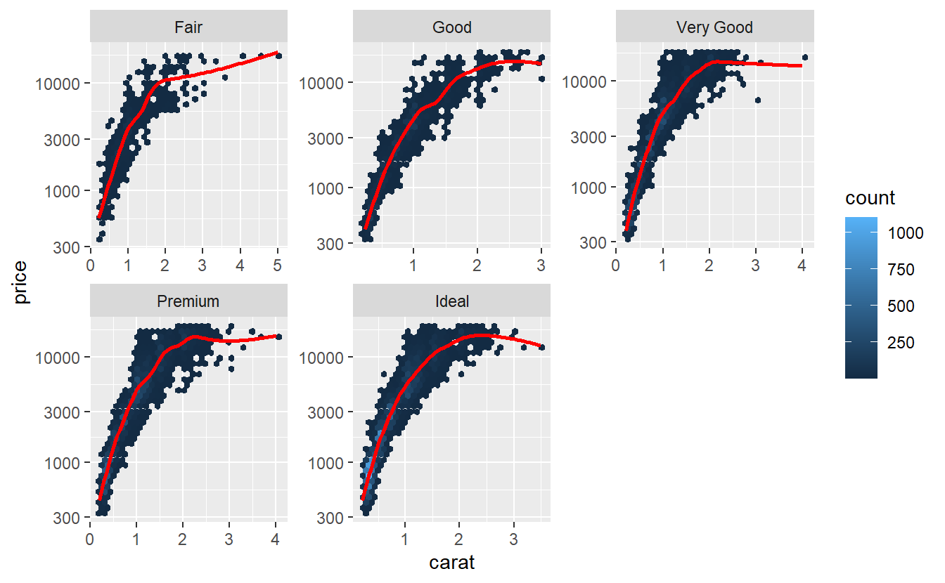
Hmm, maybe transforming the carat variable, too, may help.
tib_diam %>%
  ggplot(aes(carat, price)) +
  geom_hex() +
  geom_smooth(col = "red", se = F) +
  facet_wrap(vars(cut), scale = "free") +
  scale_y_log10() +
  scale_x_log10()
#> `geom_smooth()` using method = 'gam' and formula 'y ~ s(x, bs = "cs")'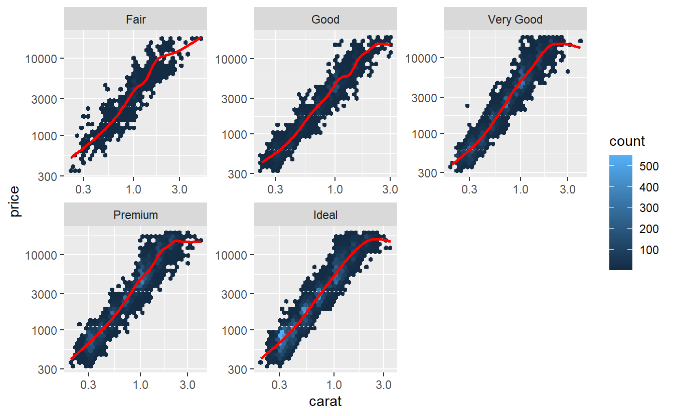
Now, this looks way better! Let’s use the transformed variables for our model.
linmod_diam <- tib_diam %>%
  mutate(cut = factor(cut, ordered = F)) %>%
  lm(data = ., log(price) ~ log(carat) + cut)
summary(linmod_diam)
#>
#> Call:
#> lm(formula = log(price) ~ log(carat) + cut, data = .)
#>
#> Residuals:
#>      Min       1Q   Median       3Q      Max
#> -1.52247 -0.16484 -0.00587  0.16087  1.38115
#>
#> Coefficients:
#>              Estimate Std. Error t value Pr(>|t|)
#> (Intercept)  8.200125   0.006343 1292.69   <2e-16 ***
#> log(carat)   1.695771   0.001910  887.68   <2e-16 ***
#> cutGood      0.163245   0.007324   22.29   <2e-16 ***
#> cutVery Good 0.240753   0.006779   35.52   <2e-16 ***
#> cutPremium   0.238217   0.006716   35.47   <2e-16 ***
#> cutIdeal     0.317212   0.006632   47.83   <2e-16 ***
#> ---
#> Signif. codes:  0 '***' 0.001 '**' 0.01 '*' 0.05 '.' 0.1 ' ' 1
#>
#> Residual standard error: 0.2545 on 53934 degrees of freedom
#> Multiple R-squared:  0.9371, Adjusted R-squared:  0.9371
#> F-statistic: 1.607e+05 on 5 and 53934 DF,  p-value: < 2.2e-16
This helped to increase our \(R^2\)-value but did not help with the additional prices of very good and premium diamonds not matching our intuition. We may take a look at the residuals of the new model:
Ok, this model looks better but still maybe outliers may be present that distort the picture. Thus, we may again try to detect them (if present) using a standardized residuals vs. fitted values plot:
# lm.influence computes leverage
hi <- lm.influence(linmod_diam, do.coef = F)$hat
res_diam <- linmod_diam$residuals
# Compute standardized residuals
n <- length(hi)
sigma <- sqrt(1 / (n - 2 - 1) * sum(res_diam^2))
standardized_res <- res_diam / (sigma * sqrt(1 - hi))

tib_diam <- tib_diam %>%
  mutate(
    res = linmod_diam$residuals,
    fits = linmod_diam$fitted.values,
    standardized_res = standardized_res
  )

tib_diam %>%
  ggplot(aes(fits, standardized_res)) +
  geom_hex() +
  geom_smooth(col = "red", se = F)
#> `geom_smooth()` using method = 'gam' and formula 'y ~ s(x, bs = "cs")'
Let us quantify how many outliers (standardized residual greater than 3 or smaller than -3) there are. If there are not too many, we can simply throw them out.
leverage_points <- lm.influence(linmod_diam, do.coef = F)$hat
n <- dim(tib_diam)[1]
tib_diam %>%
  mutate(
    outlier = ifelse(abs(standardized_res) > 3, "yes", "no")
  ) %>%
  count(outlier) %>%
  mutate(prop = n / sum(n))
#> # A tibble: 2 x 3
#>   outlier     n    prop
#>   <chr>   <int>   <dbl>
#> 1 no      53568 0.993
#> 2 yes       372 0.00690
We would lose only very little data if we threw out the outliers, so we will do that and fit the model again.
tib_diam <- tib_diam %>%
  mutate(
    outlier = ifelse(abs(standardized_res) > 3, "yes", "no"),
    cut = factor(cut, ordered = F)
  ) %>%
  filter(outlier == "no")

linmod_diam <- lm(data = tib_diam, log(price) ~ log(carat) + cut)
summary(linmod_diam)
#>
#> Call:
#> lm(formula = log(price) ~ log(carat) + cut, data = tib_diam)
#>
#> Residuals:
#>      Min       1Q   Median       3Q      Max
#> -0.76790 -0.16319 -0.00483  0.16019  0.76471
#>
#> Coefficients:
#>              Estimate Std. Error t value Pr(>|t|)
#> (Intercept)  8.203049   0.006175 1328.42   <2e-16 ***
#> log(carat)   1.698046   0.001840  922.91   <2e-16 ***
#> cutGood      0.160578   0.007107   22.59   <2e-16 ***
#> cutVery Good 0.235276   0.006588   35.72   <2e-16 ***
#> cutPremium   0.236935   0.006529   36.29   <2e-16 ***
#> cutIdeal     0.312594   0.006447   48.48   <2e-16 ***
#> ---
#> Signif. codes:  0 '***' 0.001 '**' 0.01 '*' 0.05 '.' 0.1 ' ' 1
#>
#> Residual standard error: 0.2439 on 53562 degrees of freedom
#> Multiple R-squared:  0.9419, Adjusted R-squared:  0.9419
#> F-statistic: 1.737e+05 on 5 and 53562 DF,  p-value: < 2.2e-16
Finally, these cut coefficients fit our intuition (even though the difference between very good and premium is almost nil).
Overall, we achieve a pretty high \(R^2\) value and a quick glance at the autoplot (for the sake of not having to do all plots manually, we try to compensate for the overplotting by making the points really small)
autoplot(linmod_diam, size = .05)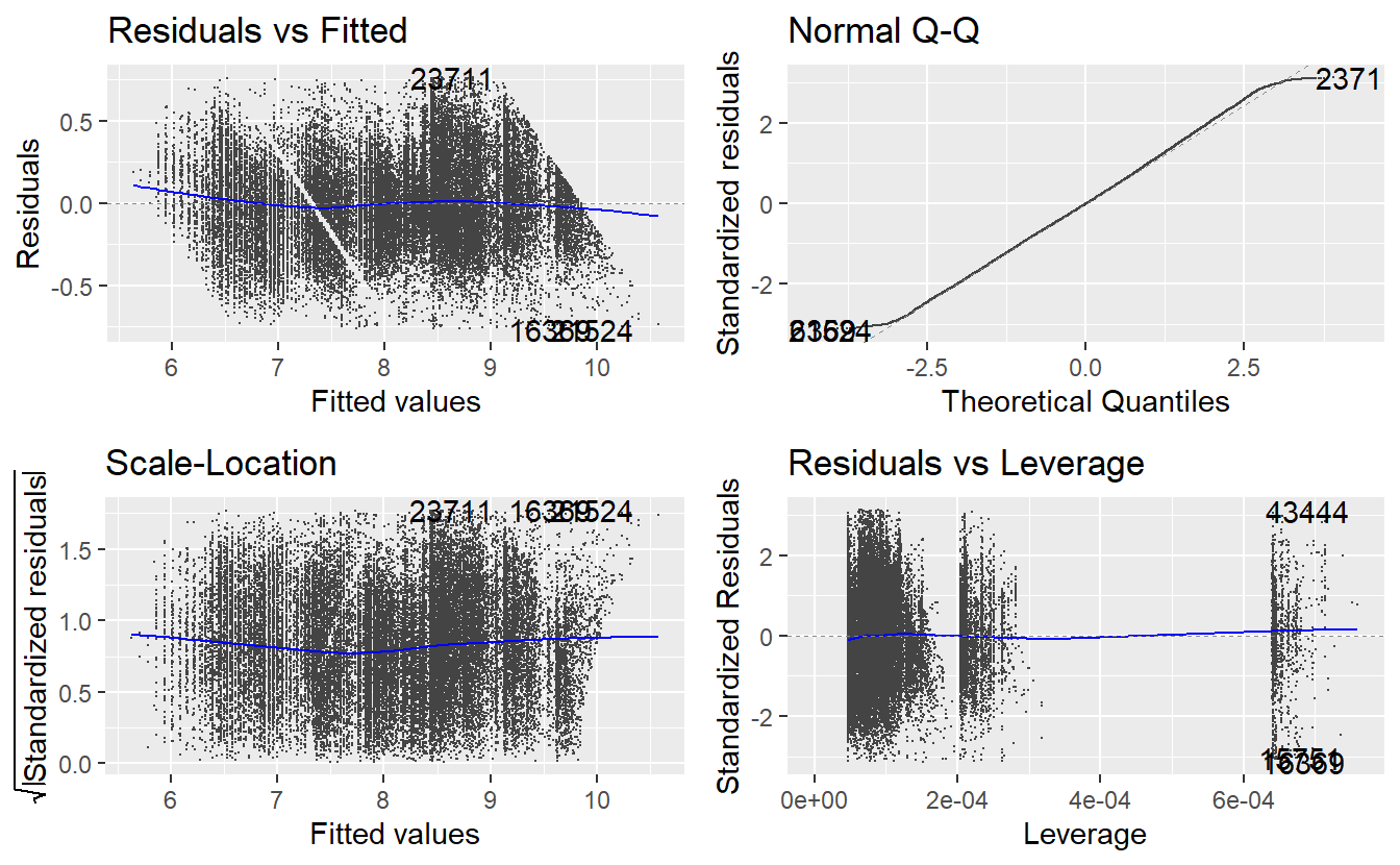
reveals that there are some outliers and leverage points which we ignore here. Other than that, the residual plots and the qq-plot look fairly decent, so we will leave the model as it is. By transforming the fitted values with the inverse of the logarithm, we can compare our model with the real observations.
tib_diam %>%
  mutate(
    model = exp(linmod_diam$fitted.values)
  ) %>%
  ggplot() +
  geom_hex(aes(carat, price)) +
  geom_line(aes(carat, model), col = "red", size = 1) +
  facet_wrap(vars(cut)) +
coord_cartesian(ylim = c(0, 22000)) 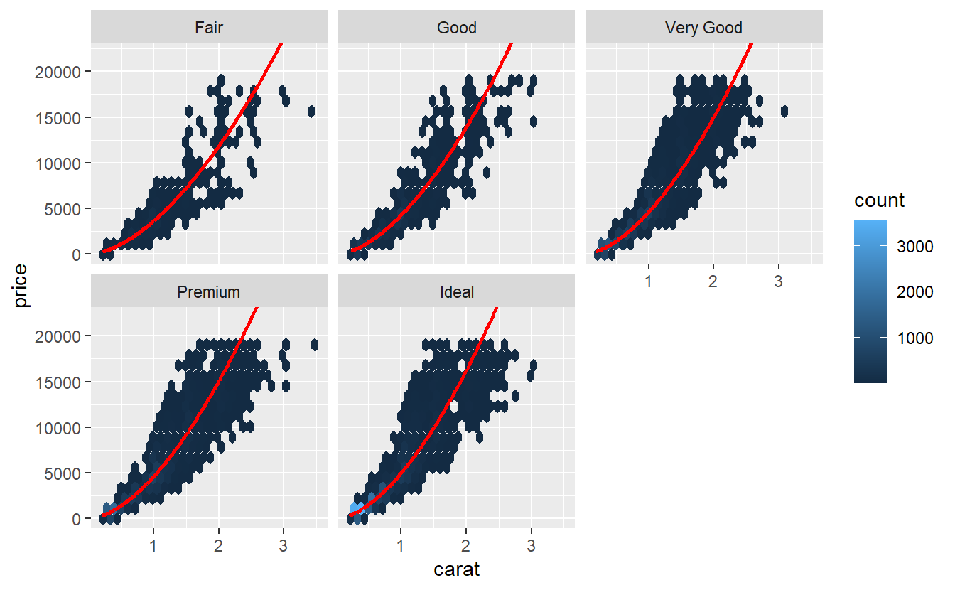
7.2.2 Confounding Variables
In the previous example, we had to deal with the fact that our model claims that the additional amount of money we have to pay for a premium diamond compared to a very good diamond of the same weight is basically nothing. This still feels odd, so we should investigate that.
In this case, a simple visualization may already reveal the problem.
To generate said visualization, the carat variable is grouped into intervals of equal length via cut_width() and boxplots depicting the distribution of the price in each interval are generated.
Finally, here it is advisable to only look at the lower 99.9% of the carat values to ignore some weird effects that occur for the top 0.01%.
diamonds %>%
  slice_min(carat, prop = 0.999) %>%
  mutate(carat = cut_width(carat, 0.2)) %>%
  ggplot(aes(y = carat, x = price)) +
  geom_boxplot()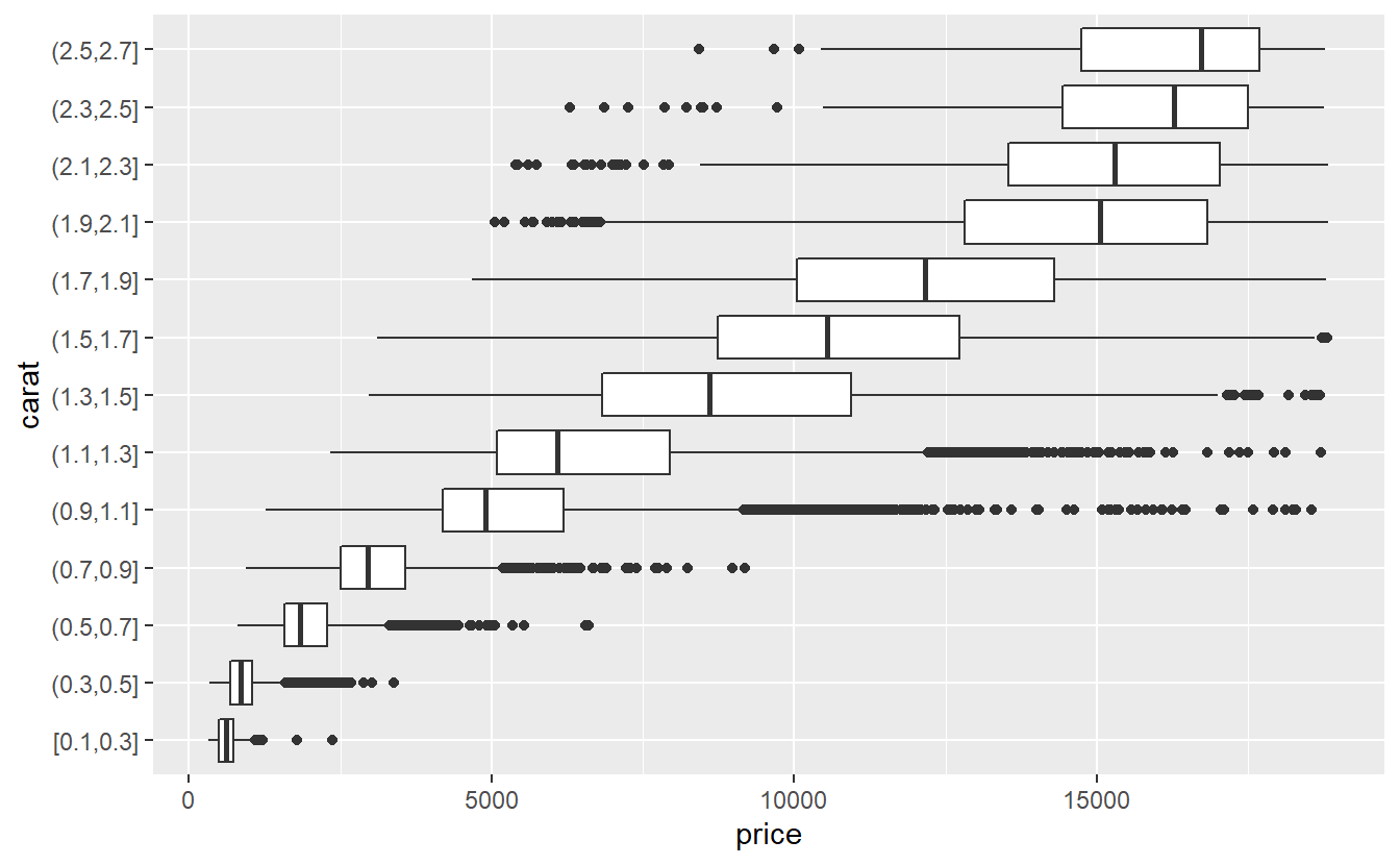
This reveals that there is a pretty obvious relationship between carat and price.
In fact, we can quantify that relationship via
cor(diamonds$carat, diamonds$price)
#> [1] 0.9215913
which constitutes a pretty strong relationship.
Now, consider the distribution of carat for each cut.
diamonds %>%
  slice_min(carat, prop = 0.999) %>%
  ggplot(aes(x = carat, fill = cut)) +
  stat_density(position = "identity", alpha = 0.25, col = "black") +
  facet_wrap(vars(cut), nrow = 5) +
  theme(legend.position = "none")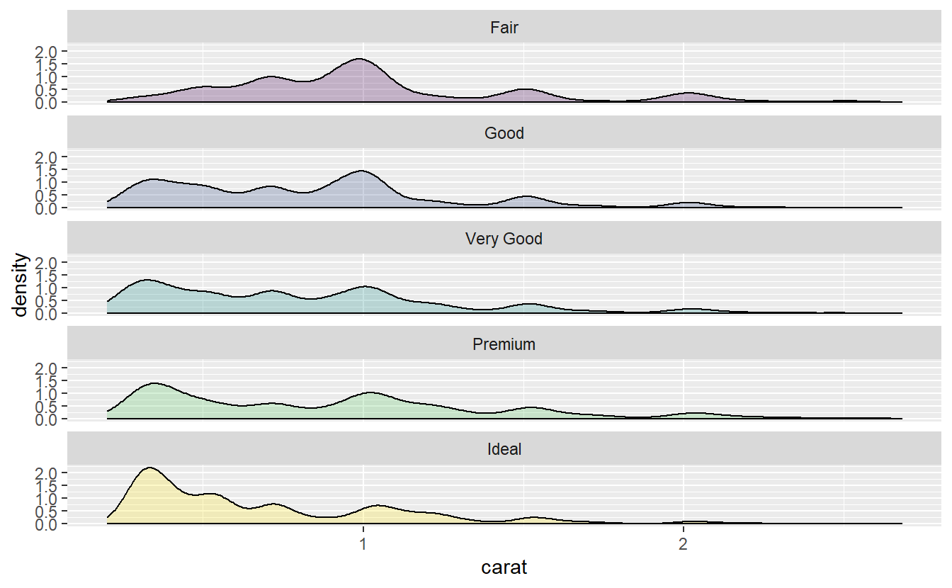
Notice that the carat distribution for the “very good” and “premium” diamonds look very similar. In fact, let us compare those two in more detail.
diamonds %>%
  slice_min(carat, prop = 0.999) %>%
  filter(cut %in% c("Very Good", "Premium")) %>%
  ggplot(aes(x = carat, fill = cut)) +
stat_density(position = "identity", alpha = 0.25, col = "black") 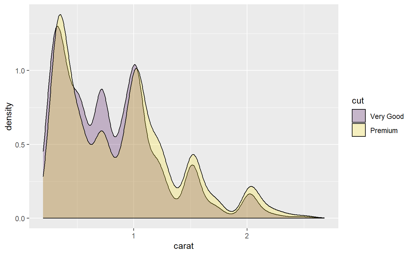
As we can see, there is a lot of overlap here.
Now, because there is such a strong association between carat and price, our linear model might also price them similarly.
Of course, from our intuitive understanding this should not happen.
Better quality should cost more.
However, our computers cannot judge like this.
They only see what is in the data.
And in this data set the variable carat influences the price quite strongly and that variable looks virtually identical for both, very good and premium diamonds.
So, our linear model will have a hard time distinguishing between those two.
This is the same reason why - if we look at the distribution of the price of the worst and best quality diamonds - it looks like the lower quality diamonds are on average more expensive.
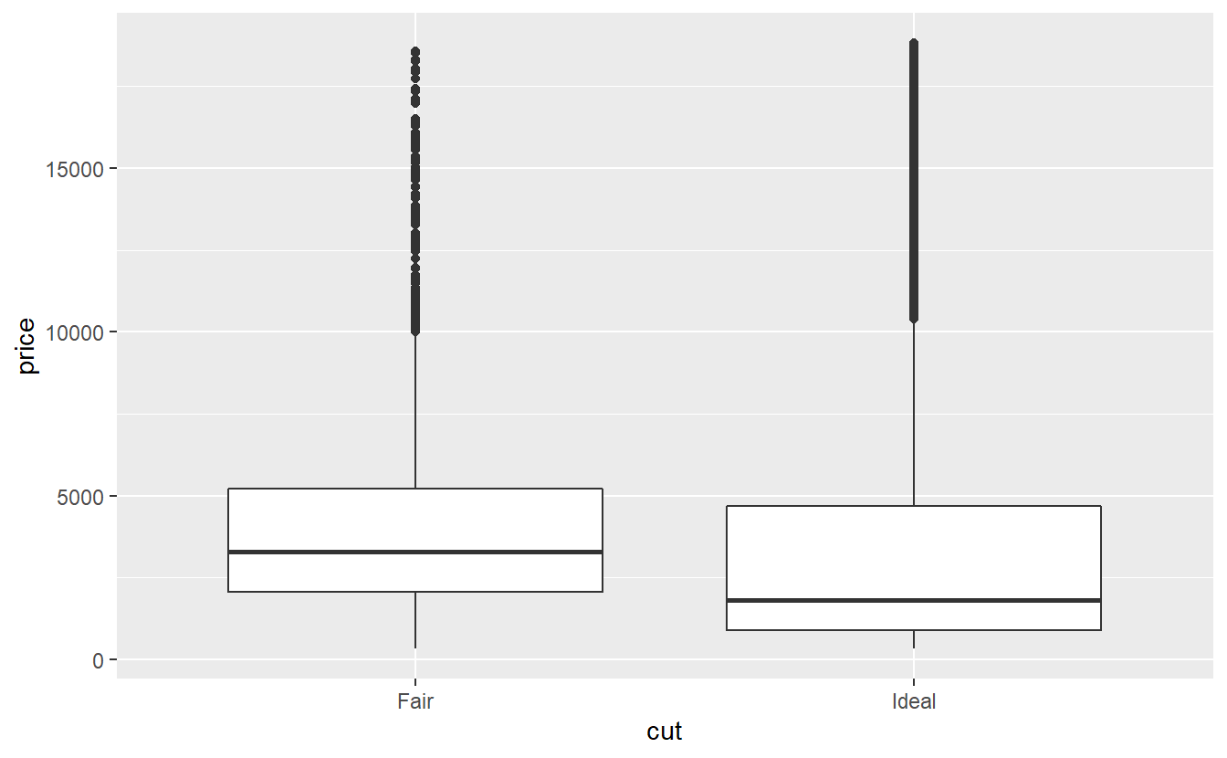
Of course, from our above density plot we can see that there are less ideal diamonds with high carats than fair diamonds with high carat.
Here, carat is what we would call a confounding variable, i.e. informally, a third variable that may obscure the relationship between two other variables.
7.2.3 Collinearity
Finally, let us briefly mention the concept of collinearity. Basically, this term describes situations where highly correlated variables are simultaneously used as predictors for linear regression. Similar to confounding, collinearity can make it hard to discern the effect of an individual variable.
In order to avoid collinearity, it can be beneficial to look at the correlation of a data set’s variables and select which variables to use or ignore for our model.
Clearly, this is only possible for numerical variables, so for our diamonds data set we can look at all variables but cut, color and clarity.
Then, we can use packages like GGally to investigate the correlation of pairs of variables.
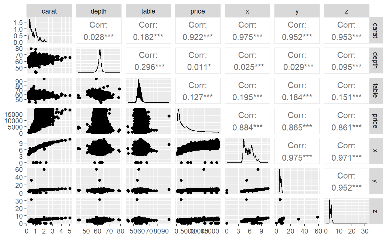
Here, we can see for each pair of variables the corresponding scatter plot and the computed correlation. Also, the diagonal entries show us a density plots of each variable.
Obviously, if either a trend is detectable in the scatter plots or the correlation is high, then we have to watch our for collinearity.
Another way to visualize the correlation is via the package ggcorrplot.
library(ggcorrplot)
cor_matrix <-  cor(diam_num)
ggcorrplot(cor_matrix, method = "circle")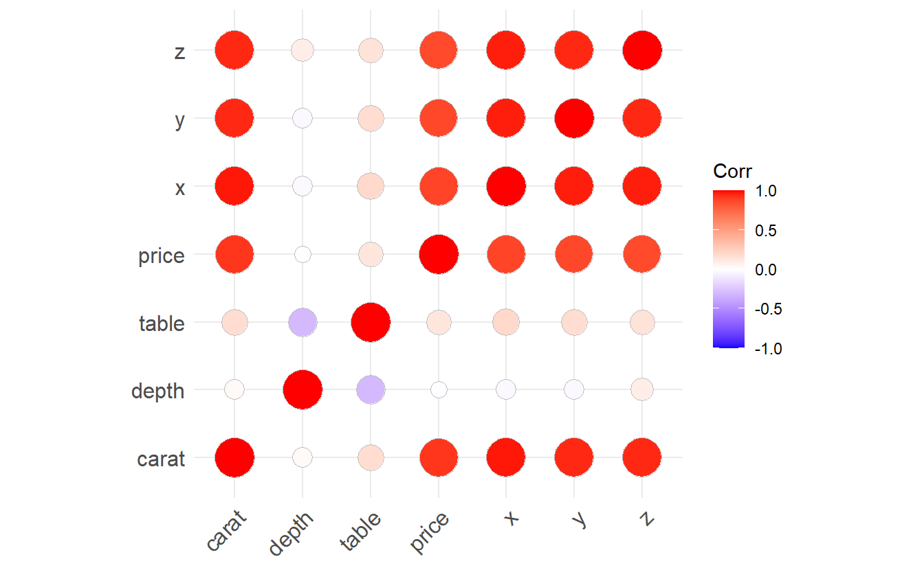
Both of the two previous plots show that each pair of carat, x, y or z is highly correlated.
Intuitively, this makes sense as x, y and z relate to length, width and depth of a diamond which of course influences a diamond’s weight carat.
Consequently, one has to be careful whether one really wants to use more than one of them as predictor.
For instance, look what happens if we use both x and carat as predictors.
diamonds %>%
  lm(data = ., price ~ carat) %>%
  summary()
#>
#> Call:
#> lm(formula = price ~ carat, data = .)
#>
#> Residuals:
#>      Min       1Q   Median       3Q      Max
#> -18585.3   -804.8    -18.9    537.4  12731.7
#>
#> Coefficients:
#>             Estimate Std. Error t value Pr(>|t|)
#> (Intercept) -2256.36      13.06  -172.8   <2e-16 ***
#> carat        7756.43      14.07   551.4   <2e-16 ***
#> ---
#> Signif. codes:  0 '***' 0.001 '**' 0.01 '*' 0.05 '.' 0.1 ' ' 1
#>
#> Residual standard error: 1549 on 53938 degrees of freedom
#> Multiple R-squared:  0.8493, Adjusted R-squared:  0.8493
#> F-statistic: 3.041e+05 on 1 and 53938 DF,  p-value: < 2.2e-16

diamonds %>%
  lm(data = ., price ~ carat + x) %>%
  summary()
#>
#> Call:
#> lm(formula = price ~ carat + x, data = .)
#>
#> Residuals:
#>      Min       1Q   Median       3Q      Max
#> -23422.7   -653.6    -14.2    370.9  12978.4
#>
#> Coefficients:
#>             Estimate Std. Error t value Pr(>|t|)
#> (Intercept)  1737.95     103.62   16.77   <2e-16 ***
#> carat       10125.99      62.55  161.88   <2e-16 ***
#> x           -1026.86      26.43  -38.85   <2e-16 ***
#> ---
#> Signif. codes:  0 '***' 0.001 '**' 0.01 '*' 0.05 '.' 0.1 ' ' 1
#>
#> Residual standard error: 1527 on 53937 degrees of freedom
#> Multiple R-squared:  0.8534, Adjusted R-squared:  0.8534
#> F-statistic: 1.57e+05 on 2 and 53937 DF,  p-value: < 2.2e-16
As you can see, the standard error of the estimate related to carat increased significantly due to collinearity.
In cases like these it is best to simply leave out the collinear variables.
This should not change too much because by their nature they bring not much new information to the table that is not already present in the other variables anyway.
We conclude this chapter by mentioning that collinearity can not only occur between a pair of variables. It is even possible to have collinearity among more than two variables. Then, we call this multicollinearity. There are ways to deal with this but these methods are outside the scope of these lecture notes.
7.3 Exercises
7.3.1 Prediction of Faster Cars
Let us take another look at the cars data set.
As you know by now, this data set contains only data on speeds up to 25 mph.
This might be cause for concern if we fit a simple linear model without quadratic term on this data and try to predict speeds that are way larger than 25.
To see what might happen, do the following:
- Fit a linear model \(\text{dist}_i = \beta_1 \text{ speed}_i + \varepsilon_i\) based on the data in
cars. - Predict the distance it takes a car to stop if it drives at \(26, 27, \ldots, 100\) mph according to your fitted model.
- Compare this to simulated stopping distances from the physical model given in Section 3.3.2. To do so, assume that residuals w.r.t. the physical model follow a normal distribution with mean 0 and standard deviation 20.
Visualize your findings and interpret the result. Also, find out how results would change if we had fitted a linear model with additional quadratic speed term (but still without intercept).
7.3.2 Interpretation of Coefficients
Suppose we fit the following two models.
tib_diam %>%
  lm(data = ., price ~ carat) %>%
  summary()
#>
#> Call:
#> lm(formula = price ~ carat, data = .)
#>
#> Residuals:
#>     Min      1Q  Median      3Q     Max
#> -8555.2  -801.0     4.0   578.8  9882.0
#>
#> Coefficients:
#>             Estimate Std. Error t value Pr(>|t|)
#> (Intercept) -2331.32      12.28  -189.9   <2e-16 ***
#> carat        7838.99      13.30   589.4   <2e-16 ***
#> ---
#> Signif. codes:  0 '***' 0.001 '**' 0.01 '*' 0.05 '.' 0.1 ' ' 1
#>
#> Residual standard error: 1447 on 53566 degrees of freedom
#> Multiple R-squared:  0.8664, Adjusted R-squared:  0.8664
#> F-statistic: 3.474e+05 on 1 and 53566 DF,  p-value: < 2.2e-16

tib_diam %>%
  lm(data = ., log(price) ~ carat) %>%
  summary()
#>
#> Call:
#> lm(formula = log(price) ~ carat, data = .)
#>
#> Residuals:
#>     Min      1Q  Median      3Q     Max
#> -3.3616 -0.2389  0.0338  0.2542  1.0861
#>
#> Coefficients:
#>             Estimate Std. Error t value Pr(>|t|)
#> (Intercept) 6.193778   0.003225  1920.6   <2e-16 ***
#> carat       1.995474   0.003493   571.3   <2e-16 ***
#> ---
#> Signif. codes:  0 '***' 0.001 '**' 0.01 '*' 0.05 '.' 0.1 ' ' 1
#>
#> Residual standard error: 0.38 on 53566 degrees of freedom
#> Multiple R-squared:  0.859,  Adjusted R-squared:  0.859
#> F-statistic: 3.264e+05 on 1 and 53566 DF,  p-value: < 2.2e-16
According to both models, how much does price (approximately) change when carat is increased by 1?
Often, one likes to use the logarithm w.r.t. base \(2\) instead of the log w.r.t. base \(e\).
Check how that would change the result and try to come up with a reason why the resulting coefficient w.r.t. carat is more convenient to interpret.
7.3.3 Gapminder
Take a look at the following linear model
gapminder::gapminder %>%
  lm(data = ., lifeExp ~ gdpPercap + pop) %>%
  summary()
#>
#> Call:
#> lm(formula = lifeExp ~ gdpPercap + pop, data = .)
#>
#> Residuals:
#>     Min      1Q  Median      3Q     Max
#> -82.754  -7.745   2.055   8.212  18.534
#>
#> Coefficients:
#>              Estimate Std. Error t value Pr(>|t|)
#> (Intercept) 5.365e+01  3.225e-01  166.36  < 2e-16 ***
#> gdpPercap   7.676e-04  2.568e-05   29.89  < 2e-16 ***
#> pop         9.728e-09  2.385e-09    4.08 4.72e-05 ***
#> ---
#> Signif. codes:  0 '***' 0.001 '**' 0.01 '*' 0.05 '.' 0.1 ' ' 1
#>
#> Residual standard error: 10.44 on 1701 degrees of freedom
#> Multiple R-squared:  0.3471, Adjusted R-squared:  0.3463
#> F-statistic: 452.2 on 2 and 1701 DF,  p-value: < 2.2e-16
Try to use visualizations to figure out how the variables in this model may be transformed to improve the \(R^2\)-statistic.
Also, check out the diagnostic plots generated by autoplot() to see if your transformation improved the plots.