10 How to Build a Model
In Chapters 7 and 9 we learned how to fit (generalised) linear models to a data set, so you may wonder why this chapter is called “How to Build a Model” as you might be inclined to think that we covered the basics of that already in the previous chapters. The truth, however, is that we have been focusing exclusively on what may be referred to as model specificication.
Sadly, model building is not as simple as throwing a statistical technique like linear regression at a data set and being done with it. Additionally, there is a lot of pre-processing and model testing to be done which is something we have neglected so far.
So, to make up for what we have been skipping, this chapter is designed to take us through a sample model building project, so that we can see what more is involved in the model building process. Moreover, on this journey we will finally get to explore more parts of the tidymodels metapackage which brings us tools to handle the most common modeling tasks.
Though, I must warn you: At first, the process from data set to final model may feel awfully complicated. With the tidymodels it involves things like “baking and preping recipes”, “setting modes and engines for model specification” etc. and the point of why it is implemented the way it is, may not become apparent in the beginning.
But in the end the implementations help us to avoid a lot of pitfalls. So it is worth adapting this methodology. Nevertheless, the tidymodels world is comparatively young and even though it is just part of any evolving programming language that syntax and procedures change over time, the tidymodels packages may be significantly affected by changes in the future. That being said, let us introduce the data set we want to work with here.
Quite often, it is not easy to get your hands on interesting real world data sets to practice data science on. But thankfully, there are at least a few sites on the interwebs that offer some data sets publicly. One of those sites is kaggle.com which is an online community designed to bring together (aspiring) data scientists and machine learners from all over the world to practice and explore models or take part in data science competitions.
Out of those data sets the kaggle community offers, probably the most infamous data set is the titanic data set from the competition of the same name. As the name implies, the given data set in that competition contains data on passengers of the famous British ship “RMS Titanic” that sank on the 15th of April in 1912. If you download the data and read the corresponding .csv-file it may look like this
library(tidyverse)
(titanic <- read_csv("data/titanic.csv"))
#> # A tibble: 891 x 12
#>   PassengerId Survived Pclass Name    Sex     Age SibSp Parch Ticket  Fare Cabin
#>         <dbl>    <dbl>  <dbl> <chr>   <chr> <dbl> <dbl> <dbl> <chr>  <dbl> <chr>
#> 1           1        0      3 Braund~ male     22     1     0 A/5 2~  7.25 <NA>
#> 2           2        1      1 Cuming~ fema~    38     1     0 PC 17~ 71.3  C85
#> 3           3        1      3 Heikki~ fema~    26     0     0 STON/~  7.92 <NA>
#> 4           4        1      1 Futrel~ fema~    35     1     0 113803 53.1  C123
#> 5           5        0      3 Allen,~ male     35     0     0 373450  8.05 <NA>
#> 6           6        0      3 Moran,~ male     NA     0     0 330877  8.46 <NA>
#> # ... with 885 more rows, and 1 more variable: Embarked <chr>
As is the intention of the kaggle titanic competition, we want to use this data set to classify passengers as either survivors or not.
Thus, the Survived column is the variable we want to predict and because it is a categorical variable, let us take the chance to bring it into an appropriate factor format.
titanic <- titanic %>%
  mutate(
    Survived = factor(
      Survived,
      levels = c(0,1),
      labels = c("Deceased", "Survived")
    )
  )
All subsequent calculations using the other variables, i.e. the predictors, are done at a later stage but for reasons we will see later, the outcome variable is transformed early on. Finally, our means of classification will be a logistic regression implemented with the help of the tidymodels package.
library(tidymodels)
#> Registered S3 method overwritten by 'tune':
#>   method                   from
#>   required_pkgs.model_spec parsnip
#> -- Attaching packages -------------------------------------- tidymodels 0.1.3 --
#> v broom        0.7.6           v rsample      0.1.0
#> v dials        0.0.9           v tune         0.1.5.9000
#> v infer        0.5.4.9000      v workflows    0.2.2
#> v modeldata    0.1.0           v workflowsets 0.0.2
#> v parsnip      0.1.5.9003      v yardstick    0.0.8
#> v recipes      0.1.16.9000
#> -- Conflicts ----------------------------------------- tidymodels_conflicts() --
#> x scales::discard() masks purrr::discard()
#> x dplyr::filter()   masks stats::filter()
#> x recipes::fixed()  masks stringr::fixed()
#> x dplyr::lag()      masks stats::lag()
#> x yardstick::spec() masks readr::spec()
#> x recipes::step()   masks stats::step()
#> * Use tidymodels_prefer() to resolve common conflicts.
10.1 Data Management
Before we can even begin to look at the data we need to be aware of one of the biggest issues in model building, namely overfitting.
To understand what we mean by overfitting, think about drawing a line through all points within our data set cars instead of fitting a linear model to the cars data set as we did before.
cars %>%
  ggplot(aes(speed, dist)) +
  geom_line() +
  geom_point()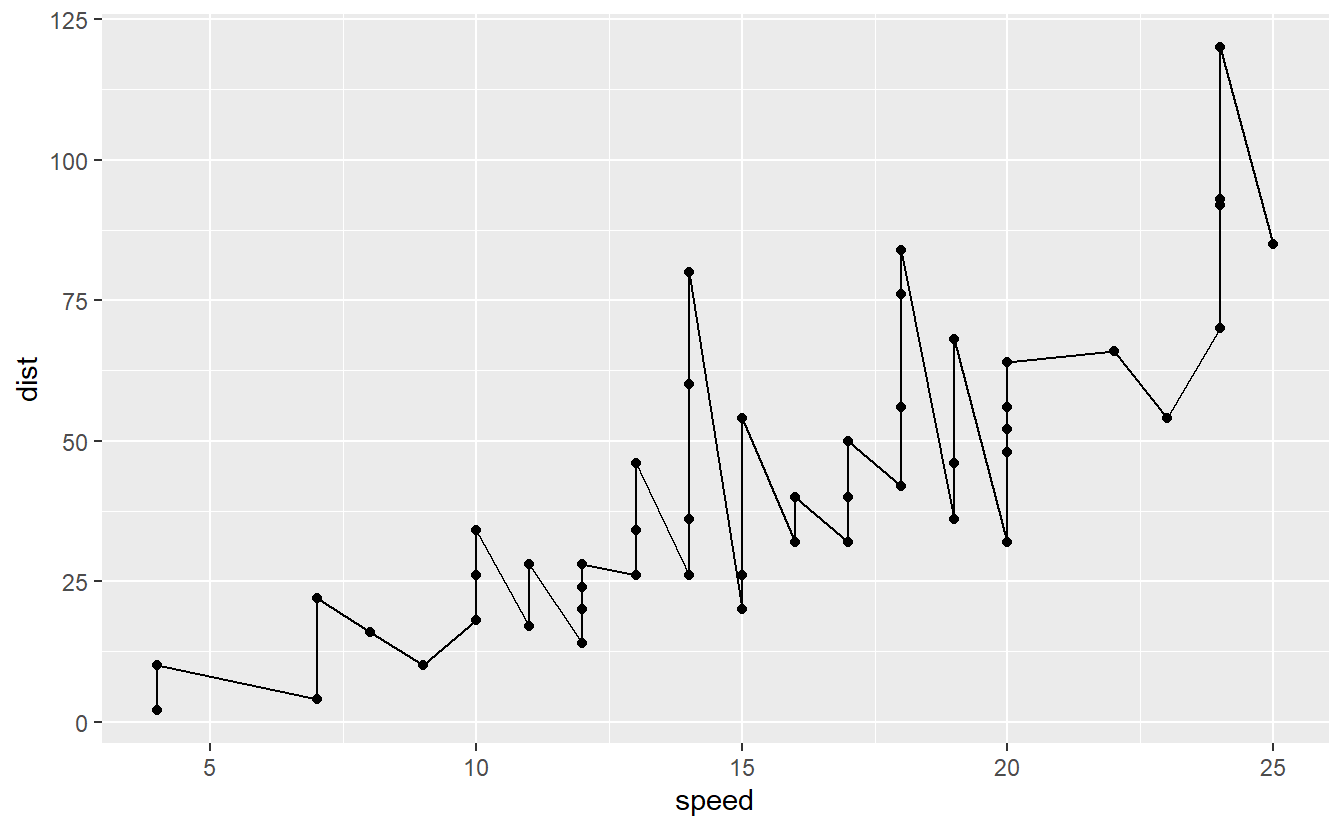
Clearly, the line that represents our “new model” is a perfect match to the data.
So, if we were to use our initial data to assess the accuracy of our model we would receive a great score.
But, of course, the model has basically zero predictive power for values of speed larger than 25.
So, while we technically have fitted a model here, it is not worth anything on data it has not seen before.
This is a clear case of overfitting where our model is “too close” to the data such that it loses its predictive power on any other data. On the other hand, consider a linear model fit.
cars %>%
  ggplot(aes(speed, dist)) +
  geom_smooth(method = "lm", se = F) +
  geom_point()
#> `geom_smooth()` using formula 'y ~ x'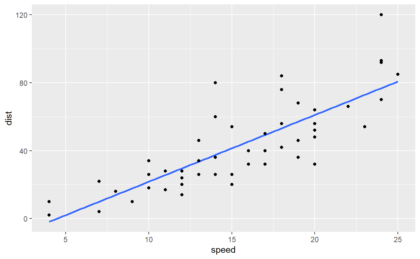
Here, we see that this model, i.e. the blue line, is less close to the data compared to our previous model. Nevertheless, this line has potentially more predictive power. Thus, the linear model sacrificed a perfect match with the underlying data, i.e. it allowed for a biased estimation and left some variation in the data unexplained (because the blue line does not perfectly track the observations) but in return gained predictive power.
Now, consider the other worst case when the model would have somewhat ignored the data like fitting a horizontal line
cars %>%
  ggplot() +
  geom_hline(yintercept = 40, col = "blue") +
  geom_point(aes(speed, dist))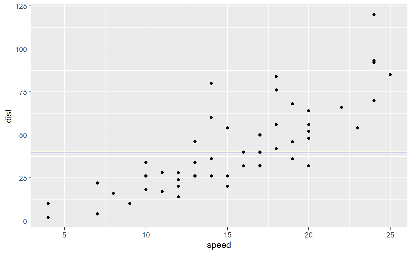
Clearly, this model is not a great fit even though it too left variation unexplained and tried not to track the data to closely. In this case, though, the bias became too large.
This conundrum of either trying to explain “too much” of the variation or “too little” of the variation is known as bias-variance tradeoff. In general, you cannot get perfect bias (i.e. no bias) and no variance which is why this is a tradeoff.
Our linear model does a decent job to find the sweet spot between variance and bias by minimizing the sum of squared residuals. So, you can think of it as having this tradeoff mechanism built into its design.
However, there are other modeling techniques such as random forests which we will cover in the next chapter that do not have such a safety mechanism, i.e. it is said that a random forest can basically learn a data set “by heart” similar to us drawing a line through all points.
If we were to test such a method on our initial data set, then regardless of the model’s predictive capabilities, our test scores would always look great. The solution to that problem comes by simply splitting our data set into training data and testing data, i.e. we use one set to fit the model and then we try to predict the observations in the testing data and see whether our model is close to the actual observations in the testing data.
Beware though that this, too, can lead to overfitting when the fitting procedure is tweaked each time when the testing scores do not show what we want to see. This is why the testing data is only used once!
Therefore, if we want to test our fitted model and possibly readjust it (which is a good idea), then we need to split our training data again. For differentiabilty, these subsets of the training data are then called analysis data and assessment data where the model is fitted on the former and evaluated on the latter set.
Even though this idea of splitting the data is quite intuitive, still things can go wrong that corrupt our analysis. For instance, imagine that we were to split our titanic data and withhold 25% (a common choice) of the data for testing. Looking at the proportions of survivors and non-survivors
titanic %>%
  count(Survived) %>%
  mutate(prop = n / sum(n))
#> # A tibble: 2 x 3
#>   Survived     n  prop
#>   <fct>    <int> <dbl>
#> 1 Deceased   549 0.616
#> 2 Survived   342 0.384
we could by accident cause our model to train with a sample that is comprised largely of non-survivors which could lead our model to underestimate the true chance of survival.
Similarly, we need to sample our data randomly.
For instance, if the data set were sorted by survivor status then taking the first \(n\) rows will, again, impact our model.
Thus, tidymodels equips of with the rsample package to make our life easier.
This brings us the function initial_split() that can also do stratified sampling which upholds the proportions of survivors and non survivors such that the proportions are the same in the testing and training data compared to the initial full data set.
However, it does not simply return two separate tibbles but bundles them in an rsplit object such that the splits are “kept together”.
set.seed(123) # Set seed for splitting
initial_split(titanic, strata = Survived)
#> <Analysis/Assess/Total>
#> <667/224/891>
Via the training() and testing() resp. analysis() and assessment() functions we can access the data from the rsplit object.
set.seed(123)
titanic_split <- initial_split(titanic, strata = Survived)
titanic_train <- training(titanic_split)
titanic_test <- testing(titanic_split)
Now, we can see that the proportions of the data was upheld. Thus, stratified sampling worked.
titanic_train %>%
  count(Survived) %>%
  mutate(prop = n / sum(n))
#> # A tibble: 2 x 3
#>   Survived     n  prop
#>   <fct>    <int> <dbl>
#> 1 Deceased   411 0.616
#> 2 Survived   256 0.384
By the same procedure we could now split the training set further, so that we can run iterations of assessing and readjusting our model. However, a common alternative is to not split the data into 2 parts but into 5 and then use 4 of those sets for analysis and the remaining set for assessment. In that way, we can actually run 5 tests on our model and get a better picture of our model performance that also accounts for randomness due to the way data is split.
This procedure is known as k-fold / v-fold cross-validation and comes with the rsample package via vfold_cv.
Again, we will have to use stratified sampling to generate the folds.
Also, the above explanation used \(k = v = 5\) but obviously we could also use \(k = v = 10\) which is the default in tidymodels.
set.seed(456) # Sampling again, so fix seed
vfold_cv(titanic_train, strata = Survived)
#> #  10-fold cross-validation using stratification
#> # A tibble: 10 x 2
#>   splits           id
#>   <list>           <chr>
#> 1 <split [599/68]> Fold01
#> 2 <split [600/67]> Fold02
#> 3 <split [600/67]> Fold03
#> 4 <split [600/67]> Fold04
#> 5 <split [600/67]> Fold05
#> 6 <split [600/67]> Fold06
#> # ... with 4 more rows
As you can see, the result of this is a tibble that contains the folds of the data, i.e. the combination of analysis set (comprised of 9 parts) and assessment set.
As before, the splits are combined in a object that is similar to the previous rsplit objects.
The model fitting procedures can deal with tibbles of folds, so we will save the folds for later on.
set.seed(456) # Sampling again, so fix seed
titanic_folds <- vfold_cv(titanic_train, strata = Survived)
10.2 Pre-processing
Now that we have split the data into training and testing data and split the training data into folds we can actually take a look at the data and see what information we have at our disposal and what we need to do to work with that.
First, we might want to check what variables are available and what variables are actually complete. So let’s do that:
| variable | NAs | prop |
|---|---|---|
| PassengerId | 0 | 0.0000000 |
| Survived | 0 | 0.0000000 |
| Pclass | 0 | 0.0000000 |
| Name | 0 | 0.0000000 |
| Sex | 0 | 0.0000000 |
| Age | 135 | 0.2023988 |
| SibSp | 0 | 0.0000000 |
| Parch | 0 | 0.0000000 |
| Ticket | 0 | 0.0000000 |
| Fare | 0 | 0.0000000 |
| Cabin | 527 | 0.7901049 |
| Embarked | 2 | 0.0029985 |
It looks like we have at least one variable PassengerId that is simply an id column which we can keep around but it won’t help us much with our classification.
Further, we have a variable Cabin that contains almost 80% missing data which, of course might be a problem.
We can either discard it, leave it as is or impute it with some value.
The same applies to the Age variable which contains only 20% missing values.
Here, I am inclined to impute the Age variable by the current median of the data. Also I might want to discard Cabin since there are really a lot of missing values.
But before we discard Cabin let’s see if maybe NAs in the Cabin variable actually relate to someone having not survived.
titanic_train %>%
  mutate(Cabin = if_else(is.na(Cabin), "Missing", "Available")) %>%
  ggplot(aes(y = Cabin, fill = factor(Survived))) +
  geom_bar(position = "fill")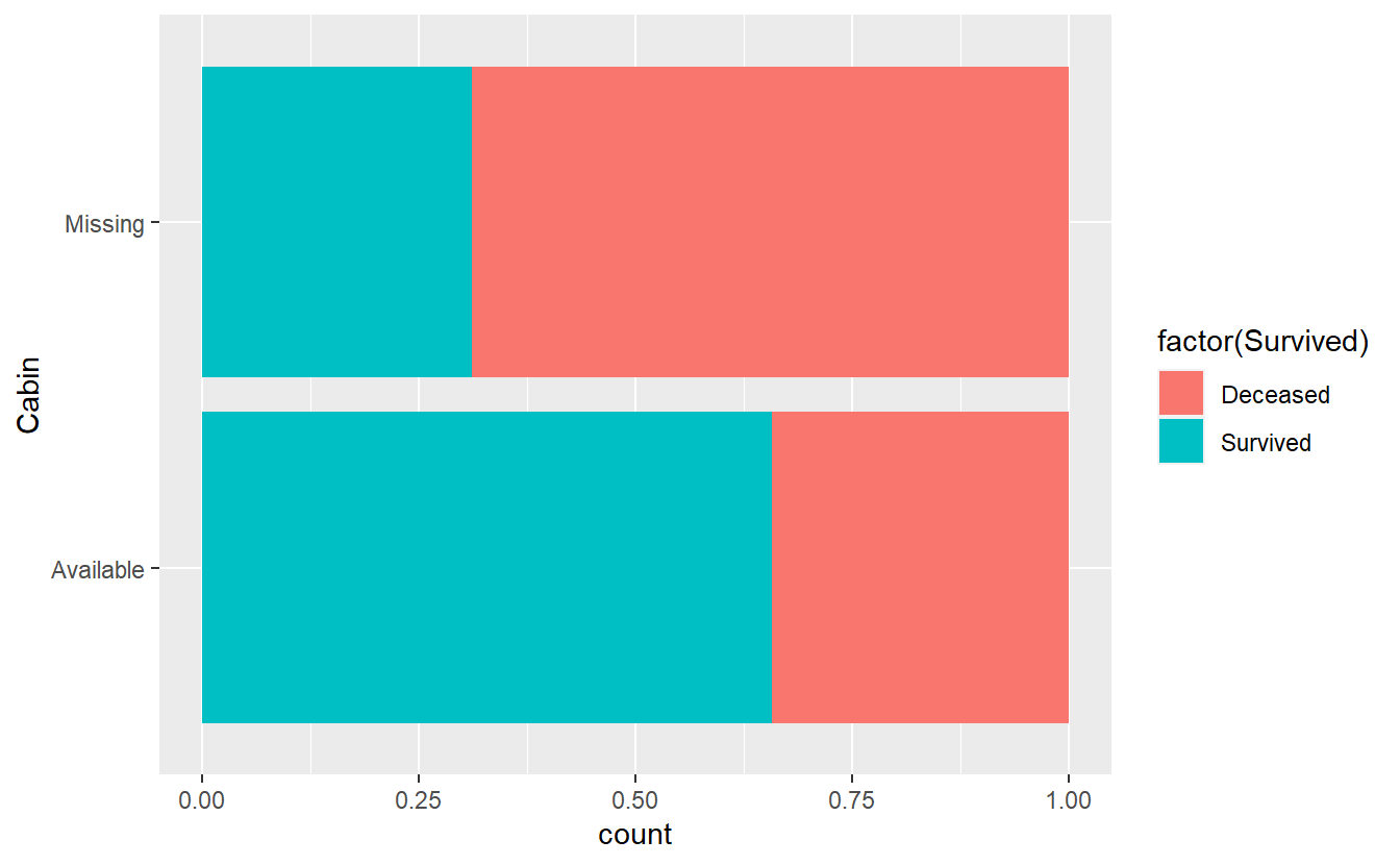
It looks like if Cabin contains some information, then it is more likely that someone survived and if Cabin does not contain any information, then it is more likely that this person has not survived.
Thus, the missing values contain some information after all.
However, we will need to encode the Cabin variable differently because usually functions do not like to work with missing values.
For simplicity, we will encode the variable as we did for the visualization even though a more fine-grained encoding w.r.t. to the available data entries could potentially make our classification better.
In summary, what we have detected at first glance is that we want to impute the Age variable and encode the Cabin variable differently.
These are classical pre-processing procedures in order to get the data ready to apply our logistic regression.
However, now the question becomes how we want to keep track of all the changes we want to make. Remember that we have many cross-validation folds on which we will need to apply the same pre-processing steps. Thus, simply making the changes to our training set won’t do.
Also, doing the pre-processing and then splitting the data is also not an option because depending on what we want to do, the pre-processing procedure needs to be trained solely on the training/analysis set.
For instance, recall that I want to compute the median of Age and use it to fill the missing values accordingly.
However, this median is computed with the training/analysis set only and applied to the testing/assessment sets. This may feel odd at first but consider the case when we want to only predict a single case. Then, a new median for the testing data could not be sensibly computed.
Similarly, the testing/assessment sets could be full of old people. Then, the imputed medians would be larger than is usually expected which could distort the model’s performance. So, long story short, we do pre-processing after spliting and we need something to keep track of our pre-processing steps such that they can be trained and applied accordingly for each cross-validation fold.
Again, here is where tidymodels comes into play.
In this case, it equips us with the recipes package which brings us recipes which is exactly what we need to keep track of the pre-processing steps.
The idea of an recipe is to let it know what our training data and what our predictors and response variables are via a formula.
So, using . to imply all variables, the most basic recipe here would look like
recipe(formula = Survived ~ ., data = titanic_train)
#> Data Recipe
#>
#> Inputs:
#>
#>       role #variables
#>    outcome          1
#>  predictor         11
Now, we can simply pass this recipe to step_* and similar functions to encode the pre-processing steps where the recipes packages has a bunch of those functions for all kinds of occasions.
To do the pre-processing steps we have discussed before, this would look like this.
titanic_rec <- recipe(formula = Survived ~ ., data = titanic_train) %>%
  update_role(PassengerId, new_role = "Id") %>%
  step_mutate(Cabin = if_else(is.na(Cabin), "Missing", "Available")) %>%
  step_impute_median(Age)
titanic_rec
#> Data Recipe
#>
#> Inputs:
#>
#>       role #variables
#>         Id          1
#>    outcome          1
#>  predictor         10
#>
#> Operations:
#>
#> Variable mutation for Cabin
#> Median Imputation for Age
Here update_role() makes sure that PassengerId does not have the role predictor anymore and is not used as such.
The remaining steps are straightforward.
Now, let us try one more common pre-processing step before we move on.
To do so, take a look at the variable Name.
The names themselves will probably not increase anyone’s chances of survival but their “title” may.
For instance, take a look at the first 10 names within our training set.
titanic_train$Name[1:10]
#>  [1] "Moran, Mr. James"
#>  [2] "McCarthy, Mr. Timothy J"
#>  [3] "Palsson, Master. Gosta Leonard"
#>  [4] "Saundercock, Mr. William Henry"
#>  [5] "Andersson, Mr. Anders Johan"
#>  [6] "Vestrom, Miss. Hulda Amanda Adolfina"
#>  [7] "Vander Planke, Mrs. Julius (Emelia Maria Vandemoortele)"
#>  [8] "Fynney, Mr. Joseph J"
#>  [9] "Palsson, Miss. Torborg Danira"
#> [10] "Emir, Mr. Farred Chehab"
There are titles like Mr., Mrs., Miss. and Master.
With the help of str_match() and regular expressions77 we can extract these titles which hopefully help us to differentiate who survives.
titanic_train %>%
  mutate(
    title = str_match(Name, ", ([:alpha:]+)\\."),
    # Look for ", [1 or more characters]."
    title = title[, 2]
  ) %>%
  count(title, sort = T) %>%
  mutate(prop = n / sum(n))
#> # A tibble: 16 x 3
#>   title      n    prop
#>   <chr>  <int>   <dbl>
#> 1 Mr       387 0.580
#> 2 Miss     139 0.208
#> 3 Mrs       90 0.135
#> 4 Master    29 0.0435
#> 5 Dr         5 0.00750
#> 6 Rev        5 0.00750
#> # ... with 10 more rows
The four most common titles are Mr, Miss, Mrs and Master.
Since title is a categorical variable, you can imagine that the computational cost may rise with each additional level to consider.
Therefore, it is often sensible to bunch rare levels together.
Here, we may label everything other than Mr, Miss, Mrs and Master as “Other”.
This can be done quite easily with step_other() and setting the threshold to say 2%.
Consequently, all levels that appear less often than 2% of the time are relabeled as “Other”.
Also, we won’t be using Name anymore, so we can update its role to something that is not “predictor” like “Id”.
This way, we still have it around for even better identification.
Finally, let us remove the variables Ticket and Embarked simply because I don’t want to deal with them here (even though they might be useful).
titanic_rec <- titanic_rec %>%
  step_mutate(
    title = str_match(Name, ", ([:alpha:]+)\\."),
    title = if_else(is.na(title[, 2]), "NA", title[, 2])
  ) %>%
  step_other(title, threshold = 0.02, other = "Other") %>%
  step_rm(Ticket, Embarked) %>%
  update_role(Name, new_role = "Id")

titanic_rec
#> Data Recipe
#>
#> Inputs:
#>
#>       role #variables
#>         Id          2
#>    outcome          1
#>  predictor          9
#>
#> Operations:
#>
#> Variable mutation for Cabin
#> Median Imputation for Age
#> Variable mutation for title, title
#> Collapsing factor levels for title
#> Delete terms Ticket, Embarked
Of course, there is more data exploration we could do to extract even more information and create new variables to consider. This is something known as feature engineering and is an incredibly important part of model building but for now let us be satisfied with what we extracted from the data.
Finally, let us conclude our recipe building with adding a few “standard” technical steps in order for our logistic regression to run smoothly. In this case we will
- convert all character predictors to factors (
step_string2factor()) - convert
Pclassto factor since it is a categorical variable even though it has numeric label (step_num2factor())78. - make sure that a previously unseen level of a factor in a testing/assessment set does not crash our calculation (
step_novel()) - encode the categorical variables via 0/1-dummy variables as is usually done when you call
lm()by hand (step_dummy()) - remove variables that contain only a single value (i.e. have zero variance) since it won’t have any predictive capability (
step_zv()) - normalize the numeric predictors such that the variables have mean zero and standard deviation one because that often improves model performance (
step_normalize())
titanic_rec <- titanic_rec %>%
  step_string2factor(all_nominal_predictors()) %>%
  step_num2factor(Pclass, levels = c("First", "Second", "Third")) %>%
  step_novel(all_nominal_predictors()) %>%
  step_dummy(all_nominal_predictors())  %>%
  step_zv(all_predictors()) %>%
  step_normalize(all_numeric_predictors())
titanic_rec
#> Data Recipe
#>
#> Inputs:
#>
#>       role #variables
#>         Id          2
#>    outcome          1
#>  predictor          9
#>
#> Operations:
#>
#> Variable mutation for Cabin
#> Median Imputation for Age
#> Variable mutation for title, title
#> Collapsing factor levels for title
#> Delete terms Ticket, Embarked
#> Factor variables from all_nominal_predictors()
#> Factor variables from Pclass
#> Novel factor level assignment for all_nominal_predictors()
#> Dummy variables from all_nominal_predictors()
#> Zero variance filter on all_predictors()
#> Centering and scaling for all_numeric_predictors()
While this may feel like a lot to keep in mind, the package usemodels actually allows you to generate recipe templates depending on your desired model.
So what do we do with this recipe?
Well, if we have decided that we have collected all necessary pre-processing steps, then we can prep() the recipe.
This will train the recipe and compute all necessary quantities such that the recipe can be applied to testing/assessment sets.
For example, this could be as simple as computing the medians in order for the medians to be used for imputation later on.
titanic_rec %>%
  prep()
#> Data Recipe
#>
#> Inputs:
#>
#>       role #variables
#>         Id          2
#>    outcome          1
#>  predictor          9
#>
#> Training data contained 667 data points and 543 incomplete rows.
#>
#> Operations:
#>
#> Variable mutation for Cabin [trained]
#> Median Imputation for Age [trained]
#> Variable mutation for title, title [trained]
#> Collapsing factor levels for title [trained]
#> Variables removed Ticket, Embarked [trained]
#> Factor variables from Sex, Cabin, title [trained]
#> Factor variables from Pclass [trained]
#> Novel factor level assignment for Pclass, Sex, Cabin, title [trained]
#> Dummy variables from Pclass, Sex, Cabin, title [trained]
#> Zero variance filter removed Pclass_new, Sex_new, ... [trained]
#> Centering and scaling for Age, SibSp, Parch, Fare, ... [trained]
After the recipe is prepared, we can bake() it and apply it on either the training data set via new_data = NULL or some other data set, e.g. new_data = titanic_test.
This will apply all pre-processing steps to the new_data argument.
Here, we can see this most obviously by the fact that new columns for the dummy variables were created and Embarked and Ticket were removed.
titanic_baked <- titanic_rec %>%
  prep() %>%
  bake(new_data = NULL)
names(titanic_baked)
#>  [1] "PassengerId"   "Name"          "Age"           "SibSp"
#>  [5] "Parch"         "Fare"          "Survived"      "Pclass_Second"
#>  [9] "Pclass_Third"  "Sex_male"      "Cabin_Missing" "title_Miss"
#> [13] "title_Mr"      "title_Mrs"     "title_Other"
10.3 Model specification
After we’re done with pre-processing, it becomes time to specify our logistic regression.
In tidymodels, this comes down to using the interface that comes with the parsnip package.
This package’s main intention is to give a unified interface for different implementations of a specific model specification79.
For example, to use logistic regressions we could call glm() as learned in the last chapter but there is also glmnet::glmnet() or LiblineaR::LiblineaR().
All of these can run a logistic regression using possibly differently named tuning parameters.
Basically, parsnip allows us to use either of these so-called engines to do logistic regression using streamlined tuning parameter names.
The logistic regression’s tuning parameters are outside the scope of these lecture notes, so we do not have to deal with those.
Nevertheless, it is worth pointing out that we could tweak these in the top-level function logistic_reg().
Then, all that is left to do is choose an engine (in our case “glm”) and for completeness’ sake set the mode to “classification” (This is the only possible option here. Other models may use either “classification” or “regression”).
titanic_spec <- logistic_reg() %>%
  set_engine("glm") %>%
  set_mode("classification")
titanic_spec
#> Logistic Regression Model Specification (classification)
#>
#> Computational engine: glm
Using our baked titanic training set, we could use now use fit() to fit our model specification to our training set, though we would have to make sure that we do not use our “Id” variables since it is saved in the recipe only and not in the baked tibble that they are not really predictors.
titanic_spec %>%
  fit(
    data = select(titanic_baked, -c(PassengerId, Name)),
    formula = Survived ~ .
  )
#> parsnip model object
#>
#> Fit time:  21ms
#>
#> Call:  stats::glm(formula = Survived ~ ., family = stats::binomial,
#>     data = data)
#>
#> Coefficients:
#>   (Intercept)            Age          SibSp          Parch           Fare
#>      -0.55037       -0.24817       -0.57133       -0.37373        0.26826
#> Pclass_Second   Pclass_Third       Sex_male  Cabin_Missing     title_Miss
#>      -0.09395       -0.50974       -7.48540       -0.33890       -6.58461
#>      title_Mr      title_Mrs    title_Other
#>      -1.82653       -5.37537       -0.59173
#>
#> Degrees of Freedom: 666 Total (i.e. Null);  654 Residual
#> Null Deviance:       888.3
#> Residual Deviance: 553.1     AIC: 579.1
As usual, we could then use predict() to see what our model predicts for a specific data set.
Here, I used the training data to see what we would get.
titanic_spec %>%
  fit(
    data = select(titanic_baked, -c(PassengerId, Name)),
    formula = Survived ~ .
  ) %>%
  predict(new_data = select(titanic_baked, -c(PassengerId, Name)))
#> # A tibble: 667 x 1
#>   .pred_class
#>   <fct>
#> 1 Deceased
#> 2 Deceased
#> 3 Deceased
#> 4 Deceased
#> 5 Deceased
#> 6 Survived
#> # ... with 661 more rows
However, since we still have our cross-validation folds titanic_folds let us use these instead for analysis and assessment of our logistic model.
Thankfully, we do not have to manually use fit() and predict() for all folds.
10.4 Workflows
With tidymodels comes another package workflows that let’s us bundle together recipes for pre-processing and model specification for modeling via so-called workflows.
In the future, it is intended that workflows can also do post-processing procedures like determining the threshold value in logistic regression (as we have done in the last chapter).
titanic_wf <- workflow() %>%
  add_recipe(titanic_rec) %>%
  add_model(titanic_spec)
titanic_wf
#> == Workflow ====================================================================
#> Preprocessor: Recipe
#> Model: logistic_reg()
#>
#> -- Preprocessor ----------------------------------------------------------------
#> 11 Recipe Steps
#>
#> * step_mutate()
#> * step_impute_median()
#> * step_mutate()
#> * step_other()
#> * step_rm()
#> * step_string2factor()
#> * step_num2factor()
#> * step_novel()
#> * step_dummy()
#> * step_zv()
#> * ...
#> * and 1 more step.
#>
#> -- Model -----------------------------------------------------------------------
#> Logistic Regression Model Specification (classification)
#>
#> Computational engine: glm
As you can see, titanic_wf is now only a container that collects all the necessary information such that we can use our model to fit and predict.
titanic_wf %>%
  fit(data = titanic_train) %>%
  predict(new_data = titanic_train)
#> # A tibble: 667 x 1
#>   .pred_class
#>   <fct>
#> 1 Deceased
#> 2 Deceased
#> 3 Deceased
#> 4 Deceased
#> 5 Deceased
#> 6 Survived
#> # ... with 661 more rows
To use our cross-validation folds, we can simply use fit_resamples() and determine a bunch of metrics that we want to collect using the folds via a metric_set().
Additionally, if we want to save the predictions, we could set control = control_resamples(save_pred = T)
fits <- titanic_wf %>%
  fit_resamples(
    titanic_folds,
    metrics = metric_set(accuracy, f_meas, mcc, sensitivity, specificity),
    control = control_resamples(save_pred = T)
  )
fits
#> # Resampling results
#> # 10-fold cross-validation using stratification
#> # A tibble: 10 x 5
#>   splits           id     .metrics         .notes           .predictions
#>   <list>           <chr>  <list>           <list>           <list>
#> 1 <split [599/68]> Fold01 <tibble [5 x 4]> <tibble [0 x 1]> <tibble [68 x 4]>
#> 2 <split [600/67]> Fold02 <tibble [5 x 4]> <tibble [0 x 1]> <tibble [67 x 4]>
#> 3 <split [600/67]> Fold03 <tibble [5 x 4]> <tibble [0 x 1]> <tibble [67 x 4]>
#> 4 <split [600/67]> Fold04 <tibble [5 x 4]> <tibble [0 x 1]> <tibble [67 x 4]>
#> 5 <split [600/67]> Fold05 <tibble [5 x 4]> <tibble [0 x 1]> <tibble [67 x 4]>
#> 6 <split [600/67]> Fold06 <tibble [5 x 4]> <tibble [0 x 1]> <tibble [67 x 4]>
#> # ... with 4 more rows
As you can see, this collects all information in a tibble full of list-like columns but there are functions such that we can easily access what we are interested in.
collect_predictions(fits)
#> # A tibble: 667 x 5
#>   id     .pred_class  .row Survived .config
#>   <chr>  <fct>       <int> <fct>    <chr>
#> 1 Fold01 Deceased        5 Deceased Preprocessor1_Model1
#> 2 Fold01 Deceased       12 Deceased Preprocessor1_Model1
#> 3 Fold01 Deceased       25 Deceased Preprocessor1_Model1
#> 4 Fold01 Deceased       32 Deceased Preprocessor1_Model1
#> 5 Fold01 Deceased       33 Deceased Preprocessor1_Model1
#> 6 Fold01 Deceased       40 Deceased Preprocessor1_Model1
#> # ... with 661 more rows

collect_metrics(fits)
#> # A tibble: 5 x 6
#>   .metric  .estimator  mean     n std_err .config
#>   <chr>    <chr>      <dbl> <int>   <dbl> <chr>
#> 1 accuracy binary     0.822    10 0.00799 Preprocessor1_Model1
#> 2 f_meas   binary     0.859    10 0.00627 Preprocessor1_Model1
#> 3 mcc      binary     0.622    10 0.0178  Preprocessor1_Model1
#> 4 sens     binary     0.883    10 0.0162  Preprocessor1_Model1
#> 5 spec     binary     0.722    10 0.0311  Preprocessor1_Model1
Now, we could use these metrics as base case for further tweaking of our preprocessing or modeling until we are satisfied with the results. Finally, we can then use the final model to train our model on the whole training data set and predict the testing data.
10.5 Exercises
10.5.1 More Fine-grained Titles
Instead of looking only at titles “Mr”, “Miss”, “Mrs”, “Master” and “Other”, consider the following groupings.
| title | n | group |
|---|---|---|
| Mr | 517 | Mr |
| Miss | 182 | Miss |
| Mrs | 125 | Mrs |
| Master | 40 | Master |
| Dr | 7 | Academic/Clergy |
| Rev | 6 | Academic/Clergy |
| Col | 2 | Military |
| Major | 2 | Military |
| Mlle | 2 | Other |
| Capt | 1 | Military |
| Don | 1 | Other |
| Jonkheer | 1 | Other |
| Lady | 1 | Other |
| Mme | 1 | Other |
| Ms | 1 | Other |
| NA | 1 | Other |
| Sir | 1 | Other |
Use these groups and titanic_train to generate the following visualization of survival probabilities. The function case_when() may be helpful.
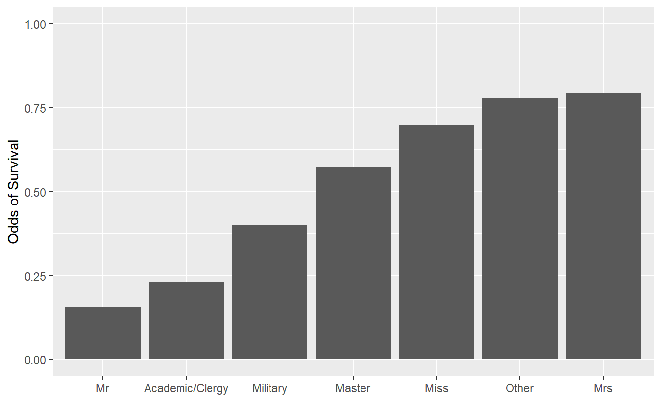
This visualization suggests that there are large differences in survival probabilities. What problems may be present with this visualization/interpretation?
10.5.2 More Fine-grained Titles II
Use these new groupings from the previous exercise to change our previous model and compare the performance of the model with the new groupings against the performance of the model with the old groupings. As before, performance is to be measured via the classification’s accuracy, F-measure, Matthews correlation coefficient, sensitivity and specificity.
Did this new grouping improve our model?
What is our model’s performance if we had not generated the variable title at all?
10.5.3 Finalize a Model
Use the function last_fit() to evaluate one of this chapter’s tweaked model by training it on the complete training set (It does not really matter which model you finalize).
Then, use the complete testing data to evaluate the model’s performance on the basis of accuracy, sensitivity, specificity and Matthews correlation coefficient.