1 Preliminaries
In this chapter, I will give a quick overview on how to install R and the highly recommended IDE2 RStudio. Afterwards, we will work our way around the RStudio interface and talk about some basic commands for R. Finally, we will learn the fundamentals of the distributed version-control system Git which makes it easier to share code and collaborate with others.
1.1 Installation of R
Before we can learn how to use R, we need to get it up and running. You can download the newest version of R for Linux, Mac or Windows from CRAN3. Once you have downloaded and installed R, you can download RStudio from RStudio’s homepage and install it as well.
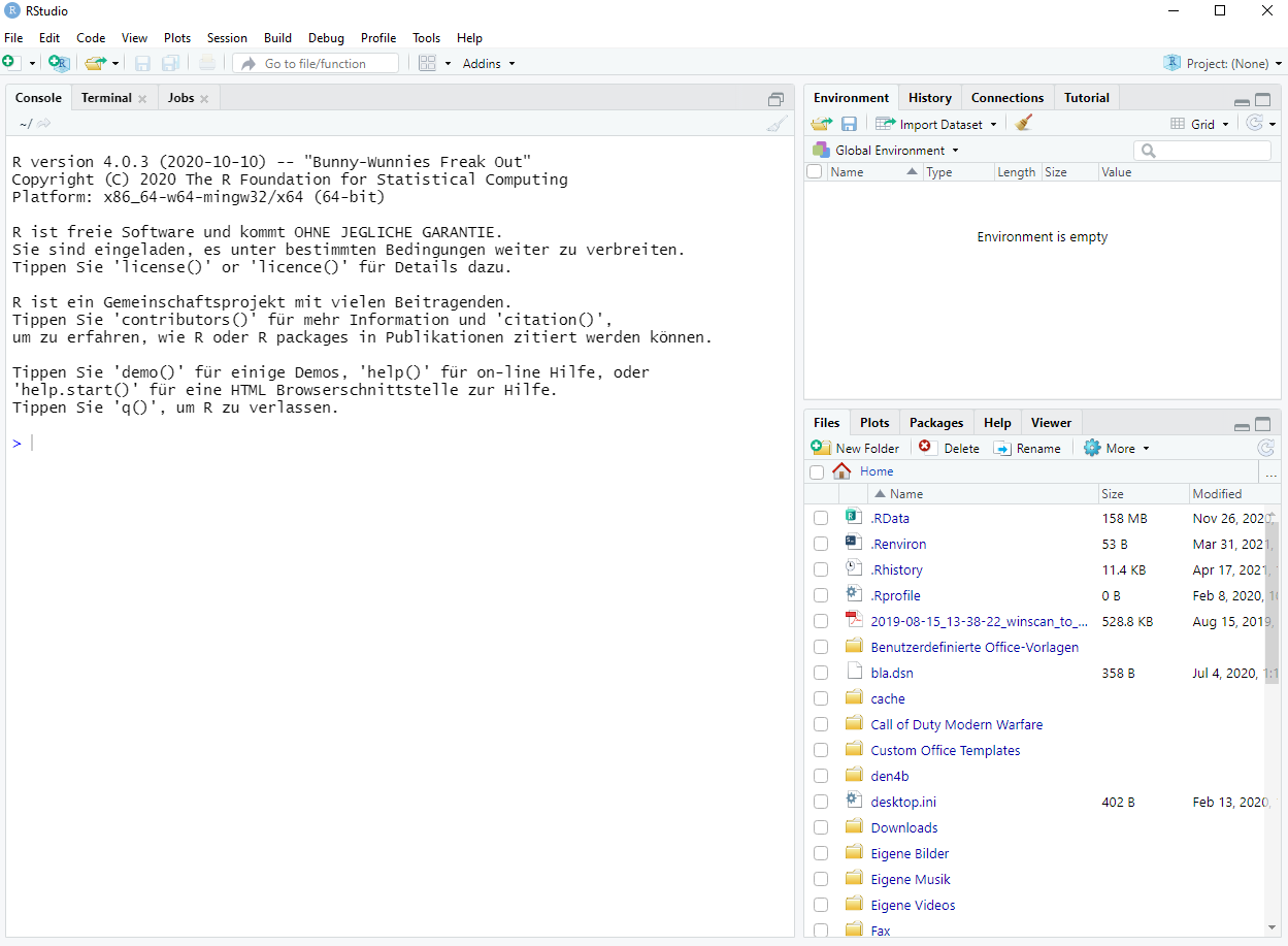
That’s more or less everything you need to get started.4 Once you have installed R and Rstudio, you can start Rstudio which then should look something like this:
We start out by using the console (the large pane on the left) to install a couple of useful packages which consist basically of a bunch of functions and/or data sets bundled together. Out of the box, R comes with a lot of functions preinstalled but there are a lot more useful functions written by other R programmers which you can access by installing the corresponding packages.
Say, you are tired and need some encouragement.
No problem, Gabor Csardi and Sindre Sorhus5 created just the right package for you.
We install the package praise by typing
install.packages("praise")into the command line of the console.
The package is now installed and does not need to be installed again when you want to use the package.
However, we will need to load the package into our current session by using the library() command.
Here, note that library() does not require "" around the package name as opposed to install.packages().
Once we have done that, we can access all functions from the praise package including the praise() function:
Oh that’s so nice of you, R.
Thanks, Gabor Csardi, Sindre Sorhus and contributors.
Alright, now that I am all motivated again, it is time to install a really useful package.
Using the same procedure as before we can install the tidyverse package by running install.packages("tidyverse") from the command line.
Then, we can load it as before using library():
library(tidyverse)
#> -- Attaching packages --------------------------------------- tidyverse 1.3.1 --
#> v ggplot2 3.3.3     v purrr   0.3.4
#> v tibble  3.1.2     v dplyr   1.0.6
#> v tidyr   1.1.3     v stringr 1.4.0
#> v readr   1.4.0     v forcats 0.5.1
#> -- Conflicts ------------------------------------------ tidyverse_conflicts() --
#> x dplyr::filter() masks stats::filter()
#> x dplyr::lag()    masks stats::lag()
As you can see, loading the tidyverse package returned an informative message, which tells us that it attached (loaded) a couple of packages.
This is due to the fact that the tidyverse is, in fact, not one single package but a collection of packages which are tailored to the needs of common tasks in data science and share a common grammar.
Loading the tidyverse attaches the core packages from the tidyverse6.
We will focus on some of the core tidyverse packages in later chapters.
For now, let me give you a short overview of some core tidyverse packages:
-
ggplot2is the graphics package of the tidyverse using the so-called layered Grammar of Graphics. We will learn more about it in Chapter 2. -
tibblebrings us tibbles for storing rectangular data, i.e. tables. Traditionally, R uses so-called data.frames for tables. You can think of tibbles as fancier data.frames. We catch a glimpse of tibbles in Chapter 2 and deal with them more thoroughly in Chapter 3. -
tidyrdelivers functions for bringing tibbles into a what we call a tidy format. We deal with tidy data in Chapter 3. -
dpylris all about manipulating and transforming tibbles. Functions from this package will be introduced in Chapter 3 and used throughout the course. -
purrrprovidesmapfunctions which allow for an efficient iteration through arbitrary tasks using “lists”. These functions are probably the hardest to learn at first which is why we will deal with them late in Chapter 8.
There are a lot more packages in the tidyverse and some are even loaded despite not showing in the message generated by library(tidyverse)7.
One notable package which is loaded but not displayed in the start up message of the tidyverse package is the magrittr package which is loaded because some of the other tidyverse packages depend on it.
The magrittr package brings us the absolutely amazing pipe operator %>% which we will learn to work with soon enough.
Let us briefly talk about the conflicts that were generated by loading the tidyverse package and then we’re all set to start working with R.
The conflicts occur due to function names appearing twice.
For instance, both the packages dyplr and stats (loaded with R startup) contain a function called filter().
Thus, because I load the tidyverse package after the stats package, the filter() function from stats is masked.
Therefore, whenever I call filter() (e.g. via the console), R will interpret my command as dplyr::filter(), i.e. calling the filter() function from the dplyr package indicated by the prefix dpylr::.
Consequently, I can still use filter() from the stats package by manually calling the function by its full name stats::filter().
This is also a very neat way to call a function from a package you have installed but do not want to load, e.g. because it might override different functions you use more frequently.
1.2 A minimum amount of R commands
This section is designed to give you a quick overview of basic R commands such as arithmetic calculations, declaring variables, vectors and tibbles. All of this is intended to give you a minimal understanding of R so that you can follow the next chapters and all other technical things about R will be covered along the way. As such, you may treat this section as a nice basis to read once without having to memorize everything and come back to it when the need arises.
1.2.1 Arithmetic Calculations and Variables
You can basically use R like a huge calculator8 and use commands such as
1 + 2                # Sum
#> [1] 3
2 - 1                # Difference
#> [1] 1
2 * 3                # Product
#> [1] 6
4 / 2                # Quotient
#> [1] 2
1001 %% 11           # Modulo
#> [1] 0

sqrt(2)              # Square root
#> [1] 1.414214
2 ^ (1 / 2)          # Square root alternative
#> [1] 1.414214
exp(1)               # Exponential function
#> [1] 2.718282
log(2)               # Natural logarithm
#> [1] 0.6931472
sin(pi)              # Sine
#> [1] 1.224606e-16
cos(pi)              # Cosine
#> [1] -1
abs(-3)              # Absolute value
#> [1] 3
sign(-3)             # Sign function
#> [1] -1
As you can see, it is possible to comment code by using #.
Everything after a # will be disregarded by R (until the next line).
Also, notice that sin(pi) did not return zero (as is the correct value) but rather an extremely small number \(1.224606 \cdot 10^{-16}\).
This is a common problem with machine precision when dealing with floating point numbers such as pi which cannot be represented with all decimal places on a computer.
There is not much we can do about this but we should at least be aware that these things can happen.
Computations can be saved into variables using <- (Shortcut in RStudio ALT + -) or =.
However, using the symbol = is discouraged as it is used as part of other functions and for the sake of separating the syntax for variable declaration and argument declaration in functions, it is encouraged to use <- for variable declaration.
sqr_root <- sqrt(100) # No outputSince a declaration does not generate an output, we have to access the variable manually to display the variable’s value.
We can do that by either calling the variable’s name or using the print() function.
A neat way to save and immediately print a variable is to put the declaration into parentheses ().
sqr_root # Output by variable name
#> [1] 10
print(sqr_root) # Output by print
#> [1] 10
(sqr_root <- sqrt(100)) # Declaration and output
#> [1] 10
Note that in instances where an output is suppressed by default (e.g. when using a for-loop which we will cover much later), the only way to force R to print a variable’s value is using the print() function.
1.2.2 Vectors
We will frequently use vectors which can be thought of as a collection of objects (e.g. numbers, characters or even other vectors). In fact, R is notoriously known for its vectorized calculations, i.e. many computations one might want to compute sequentially can actually be done in one swoop using vectors.
We can declare vectors manually with the c() function to create a collection of objects
(numbers <- c(1, 15.0, 6.3))
#> [1]  1.0 15.0  6.3

# Characters/strings are declared by using ""
(characters <- c("1001" ,"Ali", "Baba"))
#> [1] "1001" "Ali"  "Baba"

(mixed <- c(40, "Thieves"))
#> [1] "40"      "Thieves"
All of these vectors have one thing in common. They are atomic, i.e. they consist of single elements which are all of the same data type. A data type in R can be one of the following:
-
logical:TRUEorFALSE(abbreviatedTorF) -
integer: Well, integers, i.e. meaning numbers without decimal places. -
double: Any decimal number -
numeric: This is not really a data type but rather a synonym forintegerand/ordouble -
character: Characters or strings -
complex: Numeric with imaginary part -
raw: Not really of interest to us -
factor: A special format for categorical variables which allows only values from a predetermined set of level values (e.g. character valuesmale/femaleorJanuarytoDecember)
Notice that the values of the vectors mixed are in fact all of type character indicated by "" around all elements in the output.
This happens despite the fact that we used 40 (and not "40") when declaring the vector because R automatically coerces the input such that all elements are of the same type.
For obvious reasons, a character cannot be converted to a numeric in a lot of cases9, thus the default is to make the numeric become a character.
Finally, we can quite intuitively concatenate vectors by using the c() function once more
(concatenated <- c(characters, mixed))
#> [1] "1001"    "Ali"     "Baba"    "40"      "Thieves"
As suggested earlier, we could also create a vector consisting of other vectors.
To do so, we would need a different type of vectors called lists by using the list() command.
(first_list <- list(numbers, concatenated))
#> [[1]]
#> [1]  1.0 15.0  6.3
#>
#> [[2]]
#> [1] "1001" "Ali" "Baba" "40" "Thieves"numbers the way we declared it (as numeric) while the second component is of type character.
This means that we have a huge flexibility with lists as we can collect atomic vectors of different types.
However, as Uncle Ben said “With great power comes great responsibility”10, therefore we better stick to atomic vectors for now and come back to lists in Chapter 8 after we have learned to handle R better.
In summary, the vector types and their hierarchy can be summarized as follows
 licensed under [CC BY-NC-ND 3.0 US](https://creativecommons.org/licenses/by-nc-nd/3.0/us/)](Images/vector-hierarchy.png)
Figure 1.1: Vector hierarchy. Source: R4DS licensed under CC BY-NC-ND 3.0 US
1.2.3 More functions and the R Documentation
Coming back to atomic vectors, here is a collection of different ways to create vectors which will be useful later on.
vector(mode = "numeric", length = 3) # Empty numeric vector
#> [1] 0 0 0

numeric(3)                           # Shortcut for above
#> [1] 0 0 0

seq(from = 2, to = 14, by = 2)       # Sequence from-to-by
#> [1]  2  4  6  8 10 12 14

seq(from = 4, to = 6)                # Default: by = 1
#> [1] 4 5 6

4:6                                  # Shortcut for above
#> [1] 4 5 6

rep(x = 1.5, times = 4)              # Repetition of values
#> [1] 1.5 1.5 1.5 1.5

rep(x = c(1.5, 2), times = 2)        # Repetition of vectors
#> [1] 1.5 2.0 1.5 2.0

rep(x = c(1.5, 2), each = 2)         # same but elementwise
#> [1] 1.5 1.5 2.0 2.0seq() function by ?seq or in RStudio moving the cursor to a position within the string “seq” and pressing F1, we can see that the documentation looks like this
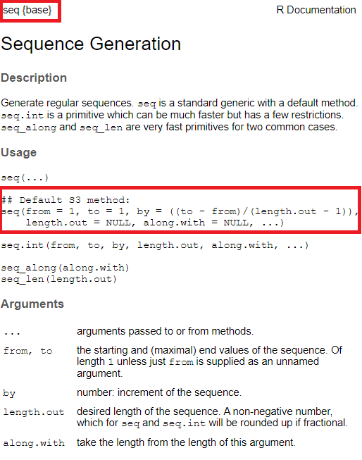
Figure 1.2: Documentation of seq()
The two red rectangles in Figure 1.2 indicate the name of functions including its package of origin (in this case base) and the default version of seq().
The R documentation is a bit messy to understand at first but essentially, here it shows that
- the first argument is
from, - the second argument is
to, - the third argument is
bywhich can be computed automatically if the argumentlength.outis used indicating how long the resulting vector should be, - there are two more arguments
length.outandalong.with, - there is a special placeholder
...that can be used for additional arguments to or from other methods.
Don’t worry if you do not fully understand every part of the documentation yet.
Usually, there are a lot of examples at the bottom of the documentation page which illustrate how a function works.
What is important here is to understand that by the default ordering of the arguments we can call seq(2, 6, 2) and R will understand it as seq(from = 2, to = 6, by = 2).
Also, we may use other arguments of the seq like so
seq(1, 2, 0.25)
#> [1] 1.00 1.25 1.50 1.75 2.00
seq(1, 5, length.out = 9)
#> [1] 1.0 1.5 2.0 2.5 3.0 3.5 4.0 4.5 5.0
Finally, two more frequently used functions are length() and seq_along().
Whereas the use case of the former function is pretty self-explanatory, the latter function deserves a small explanation.
Basically, seq_along(x) is a safe alternative for 1:length(x) (something which one might use frequently if one does not know any better11), because it does the right thing when x is a empty vector (possibly by mistake).
1.2.4 Piping
One final but highly important ingredient in our R repertoire is the so-called pipe %>%.
It is a special operator from the magrittr package in the tidyverse which helps to eliminate unnecessary intermediate variables and nested function calls.
Imagine you have a vector X full of positive integers, say
X <- c(1, 7, 5, 9, 10, 12, 8)and you want to find the maximum m of X and compute the sum of the m first even integers.12
Then, you might do that like this
# Compute the maximum, here 12
m <- max(X)

# Generate sequence of even integers
even_ints <- seq(from = 2, by = 2, length.out = m)

# Compute the sum of the sequence
sum(even_ints)
#> [1] 156
This approach involves having to save variables in between and come up with suitable variable names (which can really be frustrating if there are even more steps involved). Also, here we don’t really care about the intermediate variables. All we want is the results at the end, so why bother saving the intermediate variables.
Another approach would be to nest all the function together, resulting in one single line.
This involves having to read the code inside out, starting at max(X) and working our way outwards.
As more steps become involved this would get really messy, really fast.
One elegant alternative to both approaches involves the pipe operator %>% which sends the output of one function to another function.
If that second function knows how to deal with the output of the previous function automatically13, everything is fine.
If not, we can assist R and use the . operator to indicate how to use the previous output.
In our example this would look like this:
X %>%                     # Take X
  max() %>%               # Find the maximum
  seq(
    from = 2,
    by = 2,
    length.out = .
  ) %>%                   # Use max as length.out via '.'
  sum()                   # Compute sum
#> [1] 156
Here, we started out with our input X and sent it to the max() function which knows how to deal with a numeric vector to compute the maximum.
Then, we send that maximum to the seq() function where we specified the from and by arguments manually and told it to use the maximum as the length.out argument via the . operator.
Finally, we sent the resulting sequence to sum() for the computation of the sum.
As more steps become involved, we could easily extend this pipe by adding another %>% operator while still making sure that the code stays legible.
All in all, this is a very convenient tool which will be used frequently throughout these lecture notes.
The only drawback is that using the pipe in the console might become bothersome if one makes a mistake in one step and has to start over again line by line if one wants to incorporate line breaks in between pipe steps (which is highly encouraged for legibility). However, as we will see in the next section, we will move away from working directly with the console to working with scripts or R notebooks.
1.3 Saving and Executing R code
For our purposes, R source code comes in one of two flavors. Either your code comes wrapped in a script, i.e. an .R-file, or in a notebook, i.e. an .Rmd-File14. You can create both kinds of files using the “new file” button in the top left corner of RStudio. Once you create a new script, a new pane will open and RStudio will look similar to this:
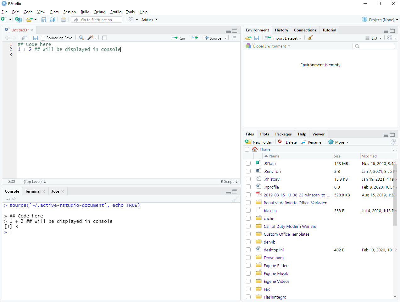
Figure 1.3: Setting up a new R script
Usually, the script is completely empty at creation. In Figure 1.3, I took the liberty of adding a few lines. Basically, you can work with scripts as if you were typing into the console and execute the script line by line. You can do this either by pressing the “run” button on each line or pressing the “source” button to execute the full script15. In a script, all results will be displayed in the console in the pane below the script.
Personally, I rarely use R scripts as much of my work is done using R notebooks because they can contain regular text and code chunks. This is only a matter of taste and depends on the situation, of course, but when trying to work with data to “figure something out”, it helps me to document my thoughts in the text part of a notebook and implement my thoughts in the following code chunk.
Consequently, if I only need to write code to accomplish a specific task, then I will work with R scripts. This is especially true when I want to execute a task on a cluster.
Naturally, this is only food for thought and you can work with whatever you prefer. If you create a new notebook it will look like this (modulo the one line of code I changed):
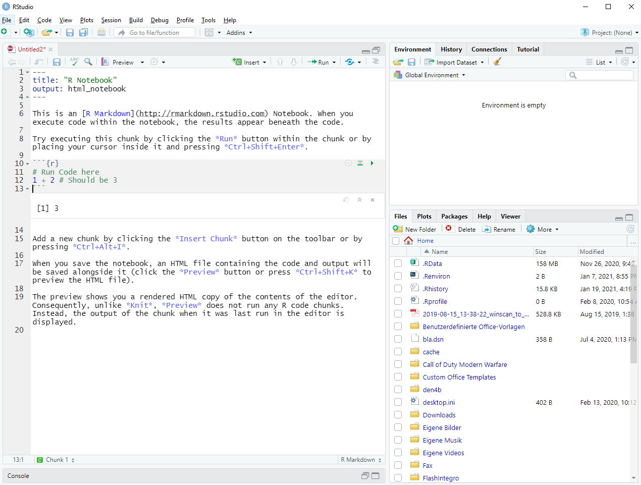
Figure 1.4: Setting up a new R notebook
As you can see in Figure 1.4 and as was already mentioned, the file contains both regular text and chunks of code (indicated by ```{r} and ```16
).
Additionally to the previous description of notebooks, let me mention that the text parts also support a lot of LaTeX commands and the notebook can easily be converted into an .html- or .pdf-file by using the dropdown menu from the “preview” button.
Now that you are able to save your code for the future you might as well learn an easy to read coding style.
For starters, I would recommend getting acquainted with the tidyverse style guide.
At this point, it is probably not useful to read all of the style guide but Chapters 2, 4 and, after our Chapter 2 on ggplot2, also Chapter 5 are recommended.
The simplest and highly effective takeaway from these chapters is the suggestion with respect to spacing, i.e. surround +, -, *, /, =, ==, <-, %>% with a single space on each side and add a single space after , (as with regular English).
Sticking to these basics will make your code more legible which will really help you in the long run.
1.4 Installation of Git
Git is version-control system and as the name implies, it allows you to switch back and forth between different versions of whatever code you’re working on. What’s more, Git is a great way to collaborate with others on the same code without the old-fashioned sending back-and-forth of emails containing the most recent changes of a file.
Originally, Git was developed for code collaboration within a software project but as you might guess from the previous description, the principles of Git can also be applied to any file that goes through numerous iterations. For instance, you could use Git to manage different versions of your thesis written in LaTeX. That way, when in doubt, you could rewrite a already written chapter and see if you are satisfied with the new form of the chapter. If not, you may simply revert to its previous version.
The only “downside” (if one may call it that) of Git is that it comes with its own unique vocabulary which can be intimidating at first. In fact, this makes it hard for new users to even search the web for solutions with respect to Git because it seems like everyone is throwing around random vocabulary.
Fortunately, I learned some of Git’s mysterious ways fairly recently, so I hope that I can address certain beginner’s questions before they even arise. For now, we will start with installation. You can download Git for your platform here. Before the installation starts, the installer will ask you about a lot of things. Just go for the default options (except for maybe when choosing Git’s default editor: There you might want to go with notepad++ instead of vim).
You can easily check if you have successfully installed Git via the shell.
For instance, you can access the shell from RStudio via Tools > Shell.
Once your shell is open, check that the following command yields a result that is not git: command not found.
git --versionOn Windows, you may have to make sure that you are on the “correct” shell, i.e. make sure that you are on the “Git Bash” shell. For this, go to Tools > Global Options > Terminal > “New terminals open with” and select Git Bash.
Next, go to GitHub and sign up for a free account there. Once you have done that go back to your shell and introduce yourself to Git via the following commands. Notice that you will need to use the email that you associated with the GitHub account you created just now.
git config --global user.name 'Otto Normalverbraucher'
git config --global user.email 'otto.n@geheim.de'
git config --global --list
The last command should then show your correct name and email. The previous two do not generate any output. Finally, in case you did not change Git’s default editor from vim to something else but still want to, you can do that via
The last step is to get a Git client to work with Git. Of course, you can work only from the shell but I seriously recommend to start your Git experience with a GUI and thus a Git client. The main advantage of a Git client is that it gives you a graphical overview of your git project and allows you to execute a lot of Git command from within the GUI.
Personally, I use GitKraken. Note however that if you want to use GitKraken as part of this course, then you will have to either buy a Pro license or get a free student pro license here as GitKraken does not allow to work with private repositories (which we will use) as part of its free plan.
Alternatively, I hear good things about SourceTree which is completely free. However, SourceTree seems to lack a merge conflict editor which comes in handy when one needs to Git cannot consolidate two different file versions automatically.
Finally, feel free to look into the vast array of other git clients to find the one git client that suits you best. On whatever Git Client you use, you will have to connect your GitHub account with your client. On GitKraken you can do that immediately after startup and on SourceTree you can add an account when you click on the “Remote” tab.
1.5 First Steps with Git
Now that you have installed Git, you are ready to learn the basics. Fortunately, you can do this interactively on Learn Git Branching. This allows me to avoid endless typing while trying to explain the steps and vocabulary of Git in full details. Chances are slim that this will help you learn Git easily because, believe me, I have tried to learned Git from those kind of texts.
Learn Git Branching helps you to learn the mechanics of Git through using (slightly simplified) Git commands and simultaneously seeing the evolving version history. Also, it offers a really simple beginners course via various scenarios and levels you can (and should) work through. The first level is depicted in Figure 1.5.
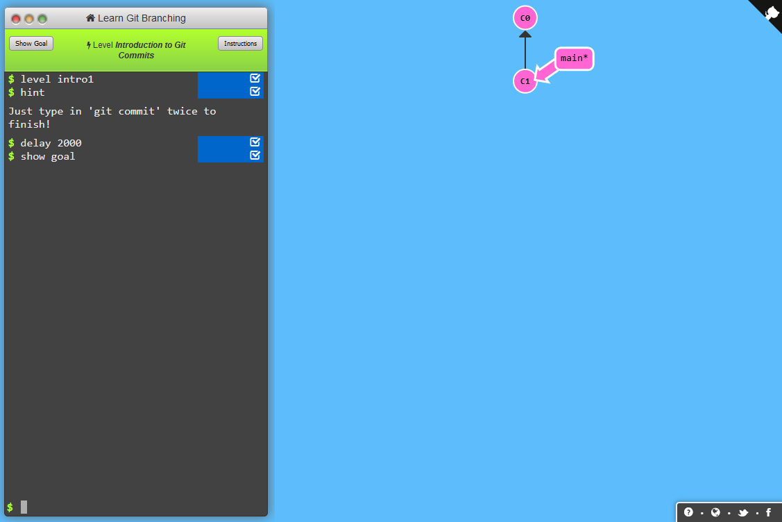
Figure 1.5: Screenshot from first level of Learn Git Branching
Therefore, I refer to the levels within Learn Git Branching to do most of the heavy lifting teaching you Git. Of course, this is not supposed to be a cheap out on my behalf. Therefore, let me give you a short primer into Git before you can run off to learn more on Git branching.
This should help you get a better picture of what it is we do with Git and what common terminology means. Even though all of the steps in this chapter can be repeated using a Git client, it can be helpful to understand what is going on behind the scenes which is why we work with the shell here. Also, to make the explanations more accessible, let us imagine that the fictional Git project we will go through in the next couple of paragraphs relates to us writing a thesis and tracking our changes.
First, let us start easy by creating a repository (or repo) on GitHub. A repo is basically where our project lives and consists of the versions we create throughout our writing process.
Log on to your GitHub account and in the top right corner, select the plus sign to create a new repository. Make sure that the repo is public and that you check the box to add a README file. Also, don’t forget to name your repository.
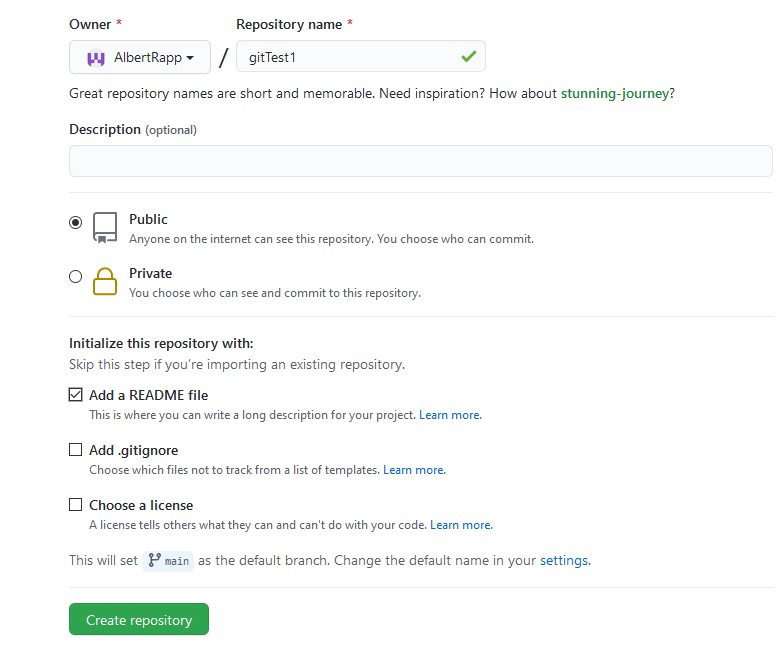
Figure 1.6: Screenshot from GitHub
In this example, I created the repository “gitTest”17. The first thing we learn about Git is that it does not necessarily store our repo solely on our computer. That is, usually there will be a local version of our data on our computer and a remote version somewhere else, e.g. on GitHub.
So far, we have created the remote version of our project, so let us clone the repository to get it onto our computer.
Copy the link of your repository, open the shell and use git clone <Link> which in my case would look like this:
git clone https://github.com/AlbertRapp/gitTest
# Cloning into 'gitTest'...
# remote: Enumerating objects: 3, done.
# remote: Counting objects: 100% (3/3), done.
# remote: Total 3 (delta 0), reused 0 (delta 0), pack-reused 0
# Unpacking objects: 100% (3/3), done.
This will copy the repo to the current working directory of your shell (you may type pwd in your git shell to find your current working directory).
Thus, we could now open the README.md file on our computer with the editor of our choice and make some changes.
For this example, I will simply add a sentence to the file and save it.
After I have done that, back on my shell I can change the working directory into the repository folder via cd and check the status of the repo via git status.
cd gitTest

git status
# On branch main
# Your branch is up to date with 'origin/main'.
#
# Changes not staged for commit:
#   (use "git add <file>..." to update what will be committed)
#   (use "git restore <file>..." to discard changes in working directory)
#         modified:   README.md
#
# no changes added to commit (use "git add" and/or "git commit -a")
This tells us that there are some changes in the repo that are not staged yet (more specifically in the README.md file).
Also, no changes have been added to a commit yet.
In Git, getting our changes ready for transfer from our local site to the remote site works in multiple steps.
From all the work we have done since the last version, we decide which changes to get to the remote site. This is the staging step.
Take a look at the changes we made. Do we really want them to become part of the version history at this point? If so, then we commit the staged changes and add a message that describes the changes. Basically, commits are the smallest unit we can work with when we want to send changes back and forth between local and remote repos.
So why do we need two steps for this? We simply do! Git works this way. It appears there are enough people on the internet that can fight over whether this is really necessary, so I will just leave you with the “best” explanation I could find: The staging area is like the pet store. Once you bring a pet home, you are committed.
So let us stage the README file via git add
git add README.md

git status
# On branch main
# Your branch is up to date with 'origin/main'.
#
# Changes to be committed:
#   (use "git restore --staged <file>..." to unstage)
#         modified:   README.md
and then commit the staged files via git commit --message "<Description>"
git commit --message "changed README file"
# [main cd428d1] changed README file
#  1 file changed, 3 insertions(+), 1 deletion(-)
Consequently, we commited to the changes we have made. Finally, we can push the commits from our local repo to our remote repo.
git push
# Enumerating objects: 5, done.
# Counting objects: 100% (5/5), done.
# Writing objects: 100% (3/3), 286 bytes | 286.00 KiB/s, done.
# Total 3 (delta 0), reused 0 (delta 0)
# To https://github.com/AlbertRapp/gitTest
#    0ad066b..cd428d1  main -> main
We could now go to our repo website on GitHub and would see (possibly after reloading the website) that whatever sentence we added to the README file is now displayed there.
Fundamentally, we just went through a typical workflow that is at the heart of Git:
- Make changes w.r.t. to one issue.
- Stage and commit work.
- Work on next issue.
- Stage and commit and repeat.
- Push commits to remote.
While these single commits feel complicated at first, this gives us the freedom to ignore commits later on. This will help us with our writing process of our thesis (remember that’s the scenario we are in here).
Let us imagine that we already completed Chapter 2 of our thesis but are not so sure anymore that the structure of Chapter 2 is okay the way it is right now. Maybe we could restructure and rewrite a couple of things and see if that is better than our original text.
Git allows us to create a branch from our current version for exactly these kind of situations.
Let’s do that using git branch <branchName>
On that branch we can go through the above cycle of making changes and committing to them. In order, to make sure our commits end up on the new branch and not on our main branch (which is the original branch of our Git project), we will have to checkout the branch.
Now that we are on the right branch, our commits may look something like this:
- Rewrite chapter intro
- Extend last paragraph of chapter
- Switch positions of section 2 and 3
- Add new figure and corresponding explanation somewhere in the middle.
Meanwhile, our original chapter is still unchanged on the main branch. Once it becomes time to decide what parts of the new branch we want to keep in your final work, we will have to get (parts of) the current branch into out main branch. We have multiple options to do so:
- Merge new branch into main branch
- Rebase new branch onto main branch
- Cherry-pick the commits we want to keep
I could probably spend a few paragraphs on each option trying to explain what is actually happening there. Point is that all of these options can bring together content from different branches. For an interactive tutorial on what happens in each options, I refer to Learn Git Branching.
Finally, let me leave you with an explanation of how GitKraken’s GUI relates to the things we did just now. This should help you even if you use a different Git client. Take a look at this screenshot I took after I merged the “newChapter2” branch into the main branch.
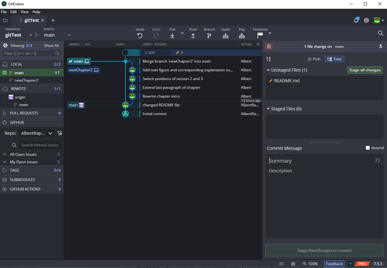
Most obviously, in the middle you can find the version history. In the “Branch / Tag” column you can see what branch is currently at what version of the documents. From this you can already infer a lot:
- The local main branch (indicated by the computer symbol) currently contains the most recent version.
- There is also a uncommited change in the files (due to me adding another sentence to
README.mdafter merging.) - The newChapter2 branch ran separatlely from the main branch (as we intended) until we merged the branch into the main branch in the most recent commit
- The remote version of the main branch, i.e. the only other present main branch,is still “stuck” on our very first change of
README.md - We are currently working on the local main branch, i.e. this branch is checked out (notice the check symbol next to the local main branch).
The nice thing about this view is the fact that I can easily see what I did in each commit. If necessary, I can revert my local files to the status after any commit by right-clicking on the commit and checking out that commit. If I want to go to a version that relates to the last version on a branch, this is even simpler and I can simply double-click on the specific branch name.
Finally, we can stage the yet unstaged changes through the pane on the right by either clicking “stage all changes” or selecting each stage-worthy line of each file. This can be done clicking on the unstaged file which will open the editor from Git where you can stage each change (which will be conveniently highlighted).
Once we have staged the desired changes, we can write a commit message in the “Summary” field on the right and hit the big green button to commit the changes.
Merging and rebasing in GitKraken is also pretty easy. Simply drag one branch name on to another branch name and GitKraken will ask you want to do. For more tips on how to use GitKraken, you may refer to Gitkraken Concepts.
1.6 Exercises
Download and install R, RStudio, Git. Optionally, you can also download and install a Git client.
SignUp with GitHub.
On Learn Git Branching, work your way through all levels of the “Main” category. Don’t worry if this looks like much, the exercises are actually pretty simple and if you are stuck you can look at the solutions.
On Learn Git Branching do all exercises of the “Remote” category except the last 6.
Try to execute the following code chunk. If you get errors, try to fix them, so that you can execute the code. If you managed to get the code running, what do you see?
library(datasauRus)
plot_data <- datasauRus::datasaurus_dozen
plot_data %>%
  filter(dataset == "dino") %>%
  ggplot(mapping = aes(x = x, y = y), col = "black") +
geom_point()- Try to change the above code chunk to plot a different data set. Available data sets are
#> away
#> bullseye
#> circle
#> dino
#> dots
#> h_lines
#> high_lines
#> slant_down
#> slant_up
#> star
#> v_lines
#> wide_lines
#> x_shape- Try to change the above code chunk to make the points have a different color instead of black. You can find a lot of color names here.